Warning: package 'ggplot2' was built under R version 4.2.2
Warning: package 'tidyr' was built under R version 4.2.2
Warning: package 'readr' was built under R version 4.2.2
Warning: package 'purrr' was built under R version 4.2.2
Warning: package 'broom' was built under R version 4.2.2
Warning: package 'dials' was built under R version 4.2.2
Warning: package 'parsnip' was built under R version 4.2.2
Warning: package 'recipes' was built under R version 4.2.2
Rows: 2455 Columns: 24
── Column specification ────────────────────────────────────────────────────────
Delimiter: ","
chr  (3): TEAM, CONF, POSTSEASON
dbl (21): G, W, ADJOE, ADJDE, BARTHAG, EFG_O, EFG_D, TOR, TORD, ORB, DRB, FT...

ℹ Use `spec()` to retrieve the full column specification for this data.
ℹ Specify the column types or set `show_col_types = FALSE` to quiet this message.
Dataset 2 (D1 college basketball)
Introduction and data
As Duke students, it goes without saying that Duke basketball adds on to our unique college experience. Noting Duke men’s basketball’s historical successes, we have grown interested in researching more about other Division 1 men’s basketball programs in universities throughout the country.
The data that we will be utilizing is sourced from the Division I college basketball seasons from the years of 2013-2019. It was found in the open source data site, Kaggle. The data was scraped from http://barttorvik.com/trank.php#. This data was cleaned up in 2021, in which the COVID seasons were not included in the dataset.
The dataset has various variables that characterize different Division I basketball teams— such as the university they represent and the conference in which they belong. Some of the observations within the dataset include the number of games played, the number of games won, power rating, as well as the stats of the team in a particular season.
Literature Review
In recent years, statistical analysis has become a critical tool for analyzing and predicting college basketball outcomes, with many researchers evaluating the relationship between offensive/defensive ratings and the performance of various basketball programs using statistical models.
Studies have revealed that offensive and defensive ratings play a significant role in a team’s success in the NCAA tournament. According to an NCAA study conducted in 2018, over nine seasons, a team’s offensive rating was about 50% more critical than its defensive rating in terms of NCAA tournament success. Another study by Bleacher Report in 2013 showed that between 2003-2013, 35 out of 40 Final Four contestants were in the top 25 in defensive efficiency, while 33 out of 40 were in the top 25 in offensive efficiency, suggesting that teams with strong defensive and offensive ratings have a higher chance of reaching the Final Four in the NCAA tournament. The most comprehensive study conducted by Albert and Bennett in 2014 examined the historical performance of NCAA men’s basketball tournament teams from 1985 to 2013 using logistic regression models, concluding that defensive performance is a significant predictor of a team’s success in the overall tournament.
Yet, while these studies and a number of others have centered around predicting the impact of offensive/defensive rating on overall tournament success, we found that very minimal research or statistical models exist analyzing the relationship between these ratings and SEED prior to the tournament, inspiring our research question and hypothesis.
Methodology
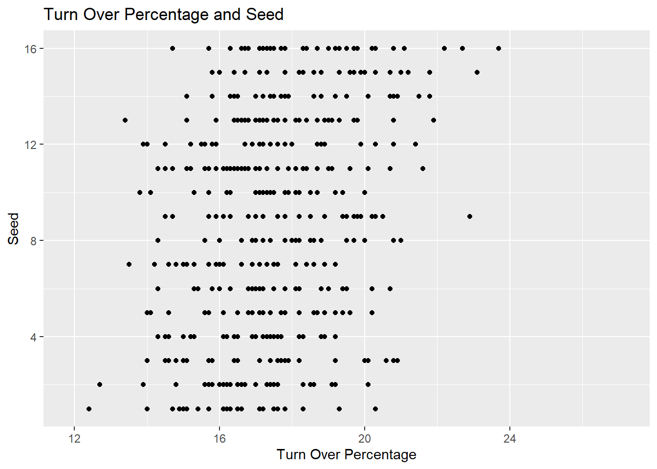
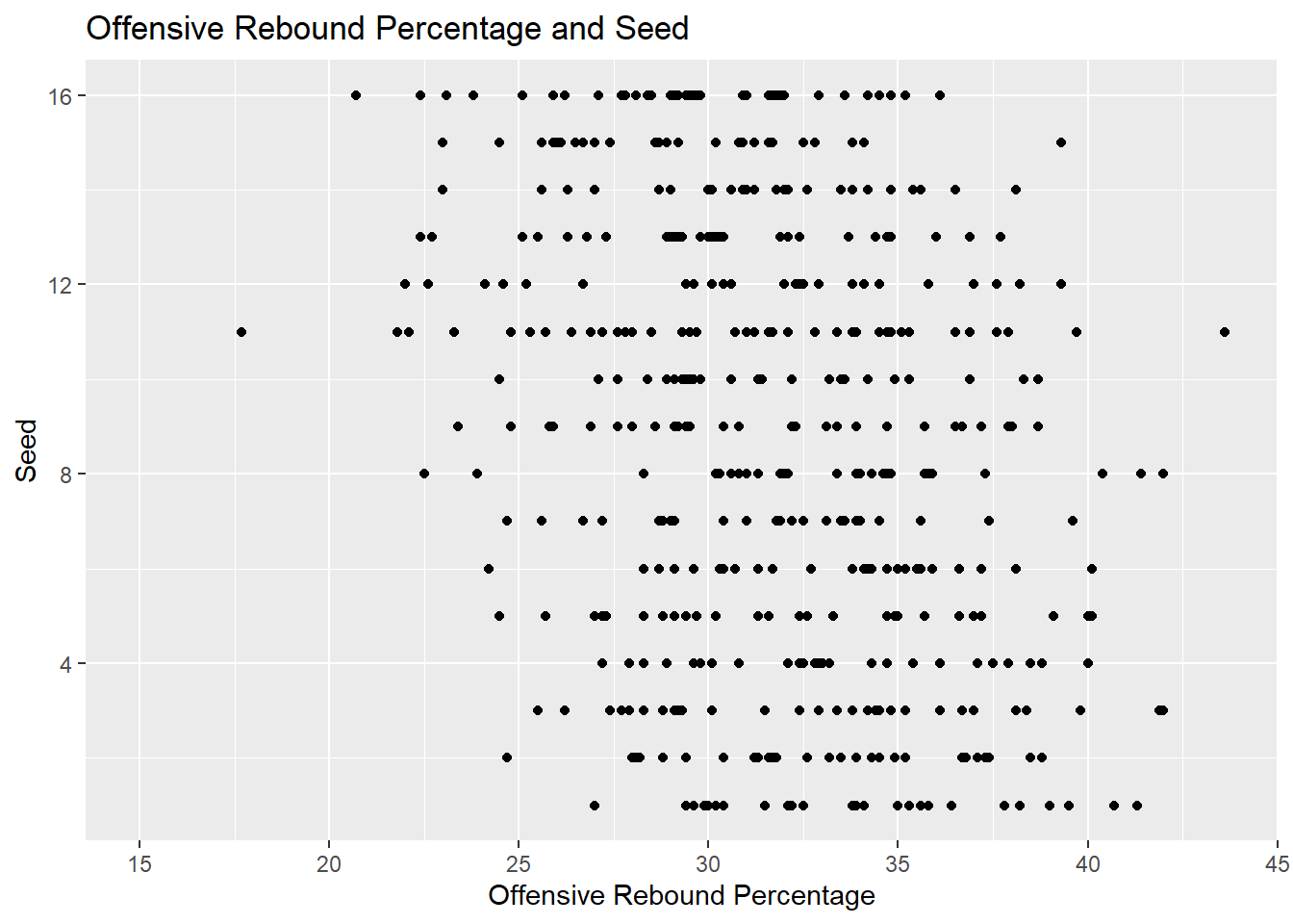
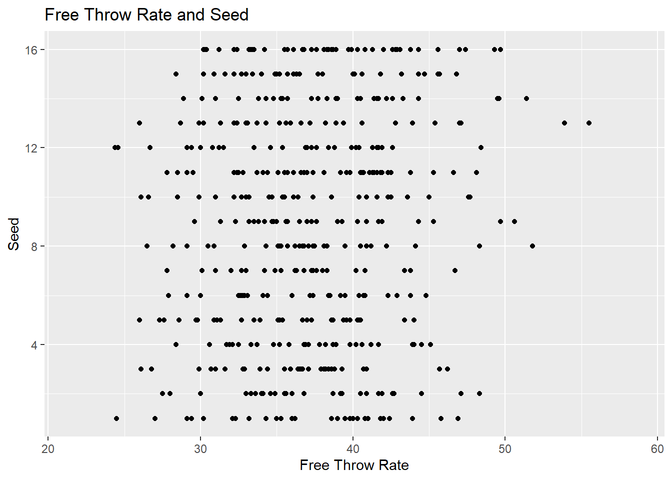
In this project, we decided to fit multiple models and find the best model at predicting postseason ranking based on season factors. For the purposes of the models we also decided to choose only teams that have made the tournament for our dataset, since we are looking at predictions for seed and not whether or not a team makes the tournament. These season factors include adjusted offensive efficiency (expected score given 100 possessions), adjusted defensive efficiency (expected opponent score given 100 possessions), Turn Over Percentage, Offensive Rebound Percentage, and Free Throw Rate. We decided based off of initial visualizations that the adjusted defensive and offensive efficiencies would be the best as they tended to have the strongest correlation to seed.
We chose to use linear regressions because we wanted to show a predicted value based on offensive and defensive efficiencies. A hypothesis test would only be able to give us an idea if they make a difference in seeding, but not be able to predict the seed. We also will then go and use adjusted r-squared which will tell us how well fit our models are to our data set while also accounting for predictors that may be insignificant (higher the better). We also will use an AIC value to compare models (from teh same dataset) since AIC is a good evaluation of if the model is a good fit for the data it was derived from and takes into account under and also over prediction of the model (lower value is better). It is also worth noting that seed is considered a numeric variable in the models and in the dataset.
Visualizations of Possible Predictors Not Used (removed data are the teams not in the tournament)
Warning: Removed 1979 rows containing missing values (`geom_point()`).
Warning: Removed 1979 rows containing missing values (`geom_point()`).
Warning: Removed 1979 rows containing missing values (`geom_point()`).
Our research question: “How does regular season adjusted offensive efficiency, and regular season adjusted defensive efficiency correlate to being a 1-seed team and post season success?”
Our central research question is addressed through the analysis of the factors that best predict overall regular season success from 2013 to 2019. We might be able to filter out the different factors that play a role in each program’s success and determine their ‘weight’ in assigning regular season rankings. With this we hope to find the best predictor for end of regular season seed given the team makes the NCAA tournament (or if the predicted seed is above 16 then they do not make the tournament).
Results
– What are you finding out?
We are finding out the best correlation between seeds and adjusted offensive efficiency/ adjusted defensive efficiency, as well as finding which predictor is the best (out of adjusted offensive efficiency, adjusted defensive efficiency, or both).
Plotting The Data
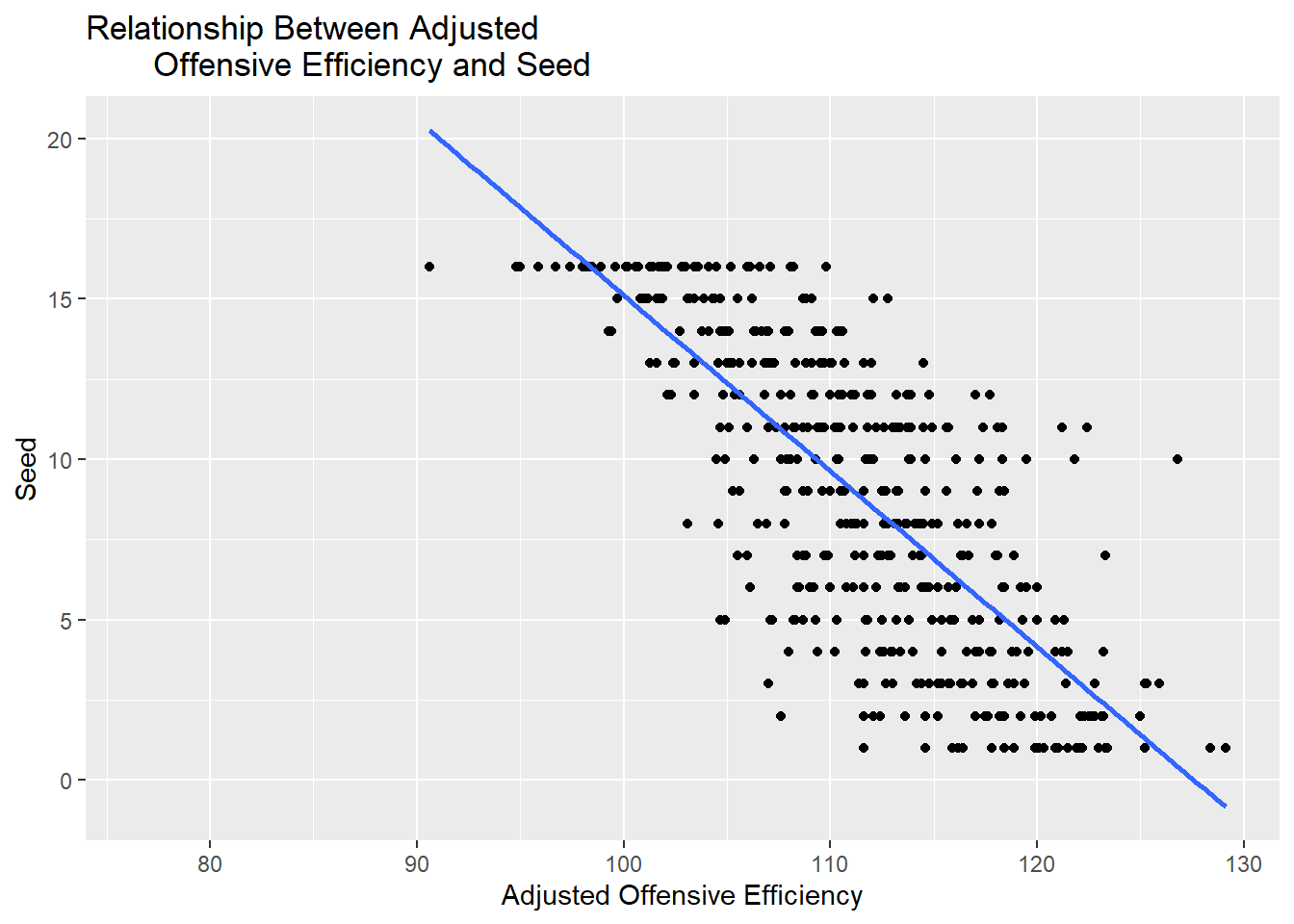
The graph above shows a strong negative correlation between seeding and adjusted offensive efficiency. This correlation shows that as adjusted offensive efficiency increases, seeding tends to also be lower (better). This outcomes makes sense, as ‘better’ teams should score more points per 100 possessions.
`geom_smooth()` using formula = 'y ~ x'
Warning: Removed 1979 rows containing non-finite values (`stat_smooth()`).
Warning: Removed 1979 rows containing missing values (`geom_point()`).
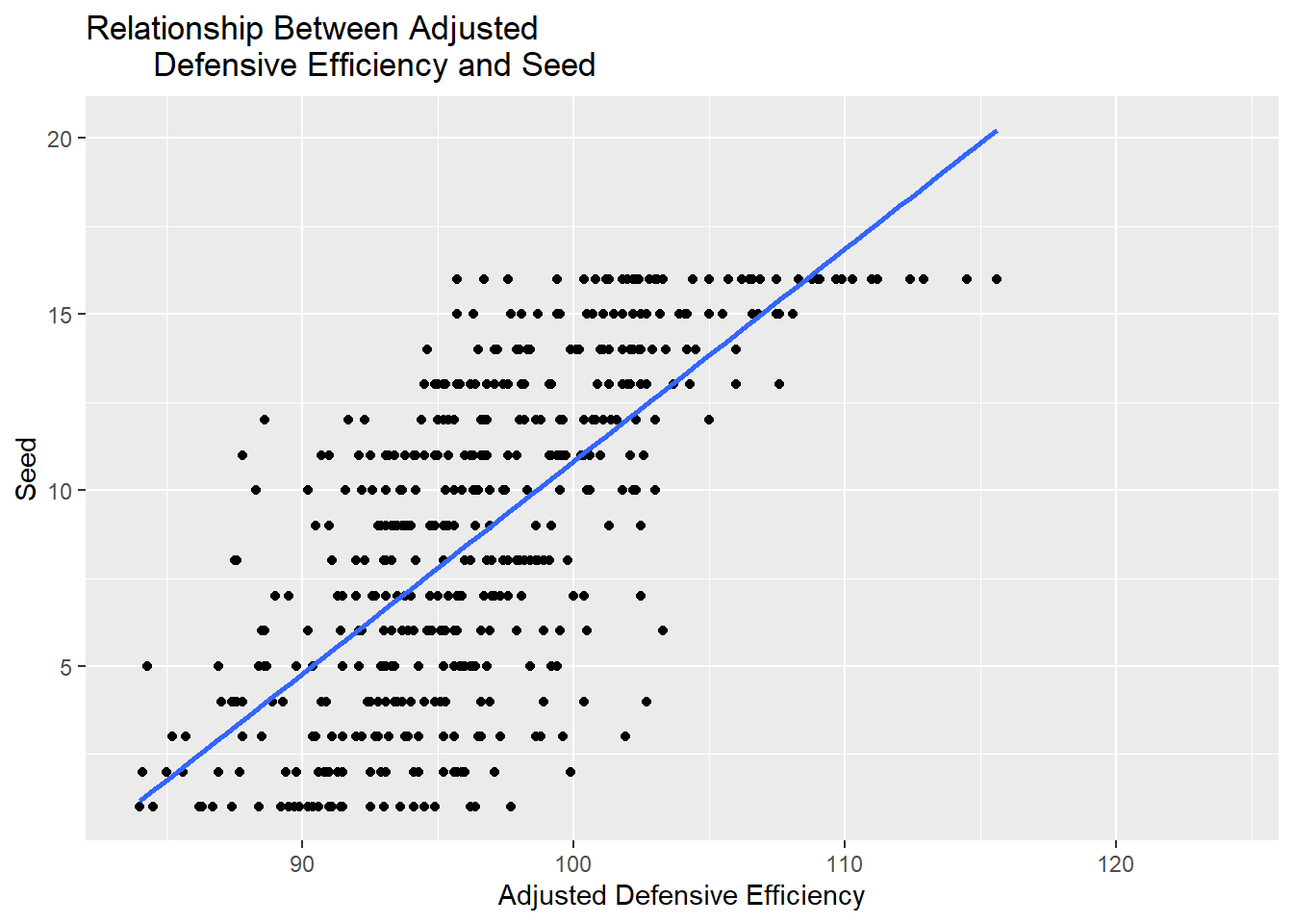
The graph above shows a strong positive correlation between seeding and adjusted defensive efficiency. This correlation shows that as adjusted defensive efficiency increases, seeding tends to also be higher (worse). This outcomes makes sense, as ‘better’ teams should not give up as many points as ‘worse’ teams per 100 possesions.
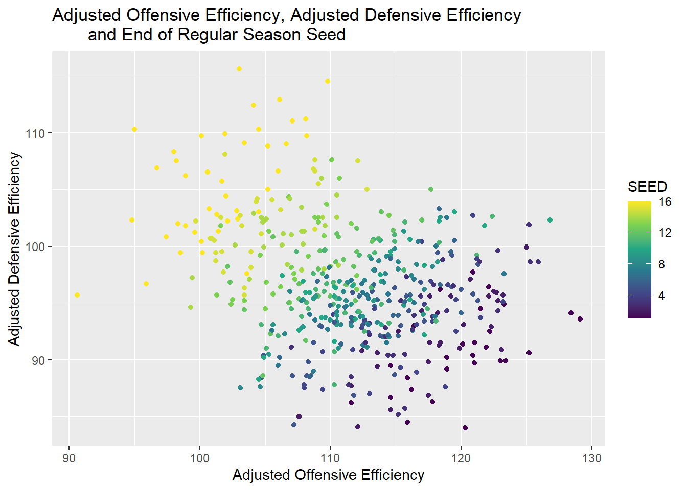
The graph above shows how the relationship that both offensive and defensive efficiency has with seed plays out. Teams with both higher offensive and lower defensive efficiencies have better seeds. This makes sense given the first two graphs, but it is also helpful to see both factors relative to seed.
Fitting Our Models
parsnip model object


Call:
stats::lm(formula = SEED ~ ADJOE, data = data)

Coefficients:
(Intercept)        ADJOE
    69.9247      -0.5482
parsnip model object


Call:
stats::lm(formula = SEED ~ ADJDE, data = data)

Coefficients:
(Intercept)        ADJDE
   -49.5214       0.6034
parsnip model object


Call:
stats::lm(formula = SEED ~ ADJOE * ADJDE, data = data)

Coefficients:
(Intercept)        ADJOE        ADJDE  ADJOE:ADJDE
  183.58562     -1.98010     -1.29158      0.01587
parsnip model object


Call:
stats::lm(formula = SEED ~ ADJOE + ADJDE, data = data)

Coefficients:
(Intercept)        ADJOE        ADJDE
    13.6156      -0.4317       0.4482
Model1 (predicting seed based on adjusted offensive efficiency)
\(\widehat{SEED} = 69.90 - 0.55*ADJOE\)
Model2 (predicting seed based on adjusted defensive efficiency)
\(\widehat{SEED} = -49.52 + 0.60*ADJDE\)
Model3 (predicting seed based on adjusted offensive and defensive efficiency [interactive model])
\(\widehat{SEED} = 183.59 - 1.98*ADJOE - 1.29*ADJDE + 0.02*ADJOE*ADJDE\)
Model4 (predicting seed based on adjusted offensive and defensive efficiency [additive model])
\(\widehat{SEED} = 13.6156 - 0.43*ADJOE + 0.45*ADJDE\)
Notes:
- we do not extrapolate data because the predictions will be extended beyond (significantly) a 16 or 1 seed
- the 3rd chart is not representative directly of our interactive and additive models.
Finding Adjusted R-Squared
Model1 (predicting seed based on adjusted offensive efficiency)
Model2 (predicting seed based on adjusted defensive efficiency)
Model3 (predicting seed based on adjusted offensive and defensive efficiency [interactive model])
Model4 (predicting seed based on adjusted offensive and defensive efficiency [additive model])
Finding AIC (Akaike Information Criterion)
Model1 (predicting seed based on adjusted offensive efficiency)
Model2 (predicting seed based on adjusted defensive efficiency)
Model3 (predicting seed based on adjusted offensive and defensive efficiency [interactive model])
Model4 (predicting seed based on adjusted offensive and defensive efficiency [additive model])
Discussion
In looking at the graphs, we can see the trend between a higher seed and the respective efficiency of offense or defense. When looking at adjusted offensive efficiency, we see as efficiency increases, seed “decreases” (approaches 1). A “lower” seed, in this case, is better. We see the opposite trend in adjusted defensive efficiency. A team seeks to have a lower adjusted defensive efficiency. In our second graph, we see that those teams with a “lower” seed have a lower adjusted defensive efficiency. This would align itself with our hypothesis. However, we want to know whether either of these predictors is better at determining seed. To do this, our models prove effective at determining this.
We have three models: one with only ADJOE, one with only ADJDE, and one with an interaction between the two. The interactive model (with both adjusted offensive and defensive efficiency) is the best model with the highest adjusted r-squared value (with the additive model just barely less accurate with a slightly lower adjusted r-squared value and a slightly higher AIC). Adjusted offensive efficiency is the third best predictor closely followed by defensive efficiency (but both are individually less correlated with their seed). This means that between offensive and defensive efficiency, adjusted offensive efficiency is slightly more important when it comes to seeding, but both combined are the most important when it comes to predicting seed. These results do match our hypothesis which again is “We predict that, in regular season, teams with higher adjusted offensive efficiency & lower adjusted defensive efficiency will be predicted to have higher seeds.”