Factors Influencing Perceived Threat in Police Violence

Investigating how race, region, and age affects the perceived threat level of an individual in a police shooting in the United States

Research Question: How does race, region, and age affect the perceived threat level of an individual in a police shooting in the United States?

Introduction/Data
Police shootings have become a pressing issue in many parts of the world, with incidents of excessive use of force by law enforcement officers making headlines and sparking widespread outrage. The consequences of police shootings can be severe, resulting in injury or death for the individuals involved and causing long-lasting trauma for their families and communities. Moreover, the use of lethal force by police can erode public trust in law enforcement and lead to social unrest, protests, and even riots. In recent years, there has been growing recognition of the urgent need to understand the root causes of police shootings and to develop effective strategies for minimizing their occurrence. 

A report by The Washington Post found that Black Americans are disproportionately impacted by police use of lethal force. Despite making up only 13% of the US population, Black Americans accounted for 24% of all people killed by police in 2020 (1). Moreover, a study by the Ruderman Family Foundation found that individuals with mental illness are also more likely to be killed by police. In fact, the report found that in some cities, such as Los Angeles, people with mental illness accounted for nearly 40% of all police shootings. Even more, according to data from the National Alliance on Mental Illness (NAMI), approximately 1 in 5 adults in the United States experiences mental illness each year; however, there are significant disparities in mental health outcomes based on race and ethnicity. For example, African Americans and Hispanic Americans are less likely to receive mental health treatment than White Americans. Additionally, research has shown that people of color are more likely to experience mental health challenges due to factors such as discrimination, trauma, and systemic racism (3).

Thus, with our data analysis, we wish to illuminate factors that impact the number of police shootings so that we can target and address ways to minimize the number of dangerous and fatal police shootings. With our research, we aim to answer how race, location, presence of mental illness, and other factors impact the prevalence of police shootings in the United States.

For our data analysis, we are using data from the CORGIS Dataset Project collected by Dennis Kafura, Joung Min Choi, and Bo Guan. This information was gathered by the Washington post in a compilation database of every fatal shooting in the United States by a police officer in the line of duty since Jan. 1, 2015. The post gathered the data by using local news reports, law enforcement websites, and social media, as well as monitoring independent databases. Using the data collected since 2015 until 2022, we can use it to predict trends and determine patterns for factors affecting the number of police shootings in the United States. While The Post conducted additional reporting in many cases, there is still a risk that the data may contain errors or inaccuracies. Moreover, the publication of this dataset could have negative consequences for the families and communities affected by these incidents. Despite these concerns, The Post updated the dataset in 2022 to provide additional information about the police agencies involved in each shooting, which could help measure accountability at the department level.

In this dataset, there are 6,569 observations. Most of these variables are categorical variables, including Factors.Threat-Level, Factors.Armed, and Factors.Mental-Illness. Some numerical variables in the dataset are Person.Age, Incident.Date.Month, and Incident.Date.Year. With this data, we can analyze the relationship between variables to look further into our reserach question and determine factors that contribute to an individual’s perceived threat level in a police shooting.

Here are links to the Police Shootings dataset from the CORGIS Dataset and More Information on the Collected Dataset:

https://think.cs.vt.edu/corgis/csv/police_shootings/

https://www.washingtonpost.com/national/how-the-washington-post-is-examining-police-shootings-in-the-united-states/2016/07/07/d9c52238-43ad-11e6-8856-f26de2537a9d_story.html

https://github.com/washingtonpost/data-police-shootings

We had three primary hypotheses. First, we hypothesized that the perceived threat level of an individual in a police shooting will be higher if the individual is a member of a racial minority group, particularly Black or Hispanic/Latinx, compared to if the individual is white. Secondly, we predicted that the perceived threat level of an individual in a police shooting will be lower if the individual is a young adult or adolescent compared to if the individual is middle-aged or older. Finally, we hypothesized that the perceived threat level of an individual in a police shooting will vary depending on the region in which the shooting takes place, with shootings in the West and Midwest regions perceived as less threatening compared to shootings in the Northeast and South regions.

We hope that our findings will encourage the urgent need to address the intersections of race, age, and other factors when it comes to police use of force. It is crucial that law enforcement officers receive proper training in de-escalation techniques and crisis intervention. Additionally, addressing the root causes of mental health disparities and systemic racism is necessary to prevent tragic outcomes and promote equity and justice. This research is crucial not only for protecting the lives and well-being of citizens but also for building stronger, more equitable, and more just societies. By studying police shootings and identifying ways to prevent them, we can work toward a safer, more peaceful future for all.

Literature Review

To contextualize our research, we examined a study entitled Examining Individual and Aggregate Correlates of Police Killings of People with Mental Illness: A Special Gaze at Race and Ethnicity. This article studies the influences of race on the existence of resistant behavior in instances of deadly police contact in people who possess mental illnesses. There are many studies focusing on civilian-police conflict, but few focus on instances in which the civilian has a mental illness and the effects of that on the encounter. In this study, they utilized regression analysis amongst, drawing upon data from the Mapping Police Violence Database.

Overall, they found that race was not a significant or consistent predictor of resistant behavior among civilians. For instance, Hispanic people with mental illnesses were found to be less likely than their White counterparts to attack the police before being killed. This is indicative of most current literature examining the influence of mental illness on police and civilian interactions, which sheds light on potential explanations for resistance and threat perception but still leaves many gaps to fill (3).

We thought this literature would be relevant to our research question as every observation in our data set is marked as having a mental illness. We thus wanted to explore further what factors affect the threat level, or indeed the perceived threat level, of individuals in a shooting.

Methodology

To begin our investigations, we tested 2 additive linear regression models to see which would most effectively predict perceived threat level. We tested using the explanatory variables of race, region, and age, and another model using the explanatory variables of fleeing, region, and age. We found the model using race, region, and age to be a better predictor of threat level because it had a lower AIC and a higher r-squared, and thus decided to move forward using this model.

To investigate the way in which race, age, and region in police shootings impact perceived threat level, we first reorganized the data set by sorting it into different American regions. We then changed some of the variables from categorical to numerical variables. To be more specific, we first mutated race into a numeric variable (1 = White, 2 = Black, 3 = Hispanic, 4 = Asian, 5 = Native American). We subsequently mutated the regions into numeric variables too (1 = Midwest, 2 = Northeast, 3 = South, 4 = West). Finally, we did the same for perceived threat level (1 = unknown, 2 = undetermined, 3 = other, 4 = attack). This is so we could more easily manipulate the data.

We then created a set of visualizations to help answer our question. We first made a bar chart looking at how the perceived threat level of an individual differed by race and region. We then made another bar chart looking more closely at the relationship between race and perceived attacks and how that changed over the years. We made a final visualization, which was a boxplot looking at the age distribution of the perceived attackers.

We fit the linear regression to encompass region, race, and age as explanatory variables and threat level as a response.

Next, we utilized the calculation of summary statistics and the predict function to isolate the effects of each explanatory variable (race, region, and age) on perceived threat level. We calculated a summary statistic to estimate the true mean of each response variable. Next, using the predict function, we utilized these means to simulate an otherwise ‘average’ individual in a shooting, only changing one variable at a time. For example, we simulated each separate race in a citizen with an average age and region.

library(tidyverse)
library(tidymodels)
library(recipes)
library(modelr)

police_shootings <- read_csv("data/police_shootings.csv")

view(police_shootings)

police_shootings1 <- police_shootings |>
  mutate(region = case_when(
    Incident.Location.State %in% c("ME", "VT", "NH", "MA", "RI", "CT", "NY", "PA", "NJ") ~ "Northeast",
    Incident.Location.State %in% c("WI", "MI", "IL", "IN", "OH", "ND", "SD", "NE", "KS", "MN", "IA", "MO") ~ "Midwest",
    Incident.Location.State %in% c("MT", "ID", "WY", "CO", "NM", "AZ", "UT", "NV", "CA", "OR", "WA", "AK", "HI") ~ "West",
    Incident.Location.State %in% c("TX", "OK", "AR", "LA", "MS", "AL", "TN", "KY", "GA", "FL", "SC", "NC", "VA", "WV", "MD", "DE", "DC") ~ "South",
    TRUE ~ "Unknown"
  )) |>
  mutate(race_num = case_when(
    Person.Race == "White" ~ 1,
    Person.Race == "Black" ~ 2,
    Person.Race == "Hispanic" ~ 3,
    Person.Race == "Asian" ~ 4,
    Person.Race == "Native American" ~ 5),
    region_num = as.numeric(factor(region)),
    threat_level_num = case_when(
      `Factors.Threat-Level` == "unknown" ~ 1,
      `Factors.Threat-Level` == "undetermined" ~ 2,
      `Factors.Threat-Level` == "other" ~ 3,
      `Factors.Threat-Level` == "attack" ~ 4
    )
  )

Visualizations

police_shootings1 |>
 ggplot(aes(x = region, fill = as.factor(race_num))) +
  geom_bar(position = "stack") +
  labs(title = "Perceived Threat Level by Race and Region",
       x = "Region",
       y = "Count",
       fill = "Race") +
  scale_fill_discrete(name = "Race",
                      labels = c("White", "Black", "Hispanic", "Asian", "Native American")) +
  facet_wrap(~ factor(ifelse(threat_level_num == 2, "Undetermined", ifelse(threat_level_num == 3, "Other", ifelse(threat_level_num == 4, "Attack", NA)))), scales = "free_y") +
  theme_minimal() +
  theme(axis.text.x = element_text(angle = 90, hjust = 1))

police_shootings |>
  ggplot(aes(x=Incident.Date.Year, fill = Person.Race)) +
  geom_bar() + 
  labs(title = "Relationship Between Race, Year, and Prevalence of Police 
       Shooting", x= "Year", y = "Number of Reported Shootings", 
       legend = "Race")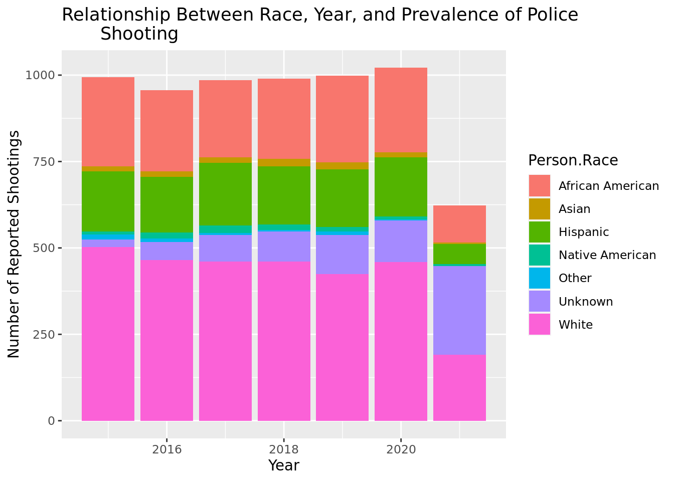

police_shootings1 |>
  filter(threat_level_num == 4) |>
 ggplot(aes(x = Person.Age, y = threat_level_num)) +
  geom_boxplot() +
  labs(title = "",
       x = "Age") +
  facet_wrap(~ factor(ifelse(threat_level_num == 2, "Undetermined", ifelse(threat_level_num == 3, "Other", ifelse(threat_level_num == 4, "Attack", NA)))), scales = "free_y") +
  theme_minimal() 

Linear Regression Model

model <- linear_reg() |>
  set_engine("lm") |>
  fit(threat_level_num ~ race_num + Person.Age + region_num, data = police_shootings1)

model

parsnip model object


Call:
stats::lm(formula = threat_level_num ~ race_num + Person.Age + 
    region_num, data = data)

Coefficients:
(Intercept)     race_num   Person.Age   region_num  
   3.623167    -0.026576     0.001993    -0.014471  

\(\widehat{threat\_level\_num} = 3.6231 - 0.0266 * race\_num - 0.0019927 * Person.Age - 0.01447 * region\_num\)

threat_level_num: {1 if unknown; 2 if undetermined; 3 if other; 4 if attack}

region_num: {1 if Midwest; 2 if Northeast; 3 if South; 4 if West}

race_num: {1 if White; 2 if Black; 3 if Hispanic; 4 if Asian; 5 if Native American}

police_shootings2 <- police_shootings1 |>
   mutate(fleeing_num = case_when(
    Factors.Fleeing == "Other" ~ 1,
    Factors.Fleeing == "Not fleeing" ~ 2,
    Factors.Fleeing == "Foot" ~ 3,
    Factors.Fleeing == "Car" ~ 4))

model2 <-linear_reg() |>
  set_engine("lm") |>
  fit(threat_level_num ~ fleeing_num + Person.Age + region_num, data = police_shootings2)

model2

parsnip model object


Call:
stats::lm(formula = threat_level_num ~ fleeing_num + Person.Age + 
    region_num, data = data)

Coefficients:
(Intercept)  fleeing_num   Person.Age   region_num  
   3.635346     0.001953     0.001736    -0.024324  

\(\widehat{threat\_level\_num} = 3.635346 - 0.001953 * fleeing\_num - 0.001736 * Person.Age - 0.024324 * region\_num\)

threat_level_num: {1 if unknown; 2 if undetermined; 3 if other; 4 if attack}

region_num: {1 if Midwest; 2 if Northeast; 3 if South; 4 if West}

fleeing_num: {1 if other; 2 if not fleeing; 3 if foot; 4 if car}

linear_reg() |>
  set_engine("lm") |>
  fit(threat_level_num ~ race_num + Person.Age + region_num, data = police_shootings1) |>
  glance() |>
  pull(AIC)

[1] 6806.318

linear_reg() |>
  set_engine("lm") |>
  fit(threat_level_num ~ fleeing_num + Person.Age + region_num, data = police_shootings2) |>
  glance() |>
  pull(AIC)

[1] 9528.969

linear_reg() |>
  set_engine("lm") |>
  fit(threat_level_num ~ race_num + Person.Age + region_num, data = police_shootings1) |>
  glance() |>
  pull(adj.r.squared)

[1] 0.007380104

linear_reg() |>
  set_engine("lm") |>
  fit(threat_level_num ~ fleeing_num + Person.Age + region_num, data = police_shootings2) |>
  glance() |>
  pull(adj.r.squared)

[1] 0.004162568

library(ggplot2)

predict_model <- police_shootings1 |>
  mutate(myPrediction = predict(model, police_shootings1)$.pred)

predict_model |>
  ggplot(aes(x = threat_level_num, y = myPrediction)) +
  geom_point() +
  labs(x = "True Perceived Threat Level", y = "Predicted Perceived Threat Level", title = "Predicted vs True Perceived Threat Level") +
  geom_abline(slope = 1, intercept = 0, color = "steelblue")

Warning: Removed 2329 rows containing missing values (`geom_point()`).

police_shootings1 |>
  summarize(mean_race = mean(race_num, na.rm = T)) 

# A tibble: 1 × 1
  mean_race
      <dbl>
1      1.67

police_shootings1 |>
  summarize(mean_age = mean(Person.Age, na.rm = T)) 

# A tibble: 1 × 1
  mean_age
     <dbl>
1     35.4

police_shootings1 |>
  summarize(mean_region = mean(region_num, na.rm = T)) 

# A tibble: 1 × 1
  mean_region
        <dbl>
1        2.96

police_shootings1 |>
  summarize(mean_threatlvl = mean(threat_level_num, na.rm = T))

# A tibble: 1 × 1
  mean_threatlvl
           <dbl>
1           3.61

predict(model, data.frame(race_num = 1, Person.Age = 35.38469, region_num = 2.960725))

# A tibble: 1 × 1
  .pred
  <dbl>
1  3.62

predict(model, data.frame(race_num = 2, Person.Age = 35.38469, region_num = 2.960725))

# A tibble: 1 × 1
  .pred
  <dbl>
1  3.60

predict(model, data.frame(race_num = 3, Person.Age = 35.38469, region_num = 2.960725))

# A tibble: 1 × 1
  .pred
  <dbl>
1  3.57

predict(model, data.frame(race_num = 4, Person.Age = 35.38469, region_num = 2.960725))

# A tibble: 1 × 1
  .pred
  <dbl>
1  3.54

predict(model, data.frame(race_num = 5, Person.Age = 35.38469, region_num = 2.960725))

# A tibble: 1 × 1
  .pred
  <dbl>
1  3.52

predict(model, data.frame(race_num = 1.670755, Person.Age = 25, region_num = 2.960725))

# A tibble: 1 × 1
  .pred
  <dbl>
1  3.59

predict(model, data.frame(race_num = 1.670755, Person.Age = 35, region_num = 2.960725))

# A tibble: 1 × 1
  .pred
  <dbl>
1  3.61

predict(model, data.frame(race_num = 1.670755, Person.Age = 45, region_num = 2.960725))

# A tibble: 1 × 1
  .pred
  <dbl>
1  3.63

predict(model, data.frame(race_num = 1.670755, Person.Age = 35.38469, region_num = 1))

# A tibble: 1 × 1
  .pred
  <dbl>
1  3.63

predict(model, data.frame(race_num = 1.670755, Person.Age = 35.38469, region_num = 2))

# A tibble: 1 × 1
  .pred
  <dbl>
1  3.62

predict(model, data.frame(race_num = 1.670755, Person.Age = 35.38469, region_num = 3))

# A tibble: 1 × 1
  .pred
  <dbl>
1  3.61

predict(model, data.frame(race_num = 1.670755, Person.Age = 35.38469, region_num = 4))

# A tibble: 1 × 1
  .pred
  <dbl>
1  3.59

Results

First, we will discuss interpretations of our four visualizations.

Our first visualization shows that nearly 2000 perceived attacks took place in the South and nearly 1500 of the perceived attacks took place in the West. This second detail was surprising to us, especially in tandem with the very low numbers of perceived attacks in the Northeast. We had hypothesized greater rates of perceived attacks in the Northeast given that Northeastern cities like New York and Baltimore are big crimes cities. This may, however, reflect the size of the West.

The relationship between race and perceived threat level was more in keeping with what we expected. Across all regions, white people made up the majority of perceived attacks, followed by African American people. While we did hypothesize that white people would not see the highest numbers of perceived attacks, and this result could thus be quite surprising, it must be noted that white people make up about 58% of the nation in contrast to African Americans who make up 13% and Hispanic people who make up 18%. In this way, it seems clear that African Americans are disproportionately targeted and race may be a predictor of perceived threat level. A considerably greater proportion of perceived attackers were African American in the South and this is perhaps indicative of stronger racial prejudices in the region.

In our second visualization, we explored the relationship between race and perceived attacks more closely. It shows that proportions of races were roughly consistent over the years. Notably, the number of threats went down significantly in 2021. This is partly due to the fact that the 2021 data was collected up to September 2021. But there are fewer than 3/4 of previous years’ threats , so the overall rate of perceived attacks did go down. The proportion of African American perceived attacks also went down. This is likely in reaction to the Black Lives Matter movement which criticized police discrimination against black people. This again suggests race could be a factor in terms of whether someone is perceived as a threat, suggesting that bias is at play. 

Our third visualization showed which ages are more likely to be perceived as a threat. Unsurprisingly, the interquartile range of perceived threats was between 25-45 and much of the older threats were counted as outliers. Given that people of ages 25-45 are more able-bodied, it makes sense that they would be perceived as more threatening. Thus, age too is an important factor in determining threat level.

Our visualization comparing the true perceived threat level and the predicted perceived threat level reveals that most of the perceived threat levels for our model appear to occur around 3-4, which means they are between undetermined and attack. This makes sense with our data because most of the observations in the dataset are “undetermined” and “attack” observations. Furthermore, the true perceived threat level points appear at fixed levels, at 2, 3, and 4 because those were categorical variables manipulated to numeric variables. Thus, we would not visualize any data points in between 2, 3, and 4 because they are fixed values at those integers.

But visualizations are not the most accurate way of answering our question. We therefore looked to further methods.

Next, we investigated the individual effects of each variable, utilizing the predict function. Our predict model investigating race produced fairly inconclusive results, but this can in part be explained by the disproportionate racial population distribution. The perceived threat levels were all fairly similar, with 3.62426 for White, 3.597684 for Black, 3.571108 for Hispanic, 3.544532 for Asian, and 3.517956 for Hispanic. However, when we consider sample sizes differences due to discrepancies in population, this highlights that we do not conclude that White people are more likely to be perceived as a threat than racial minorities.

Next, we investigated age, employing an average race and region numeric value to hold those factors constant. I based test ages around the mean, which was 35, utilizing 25, 35, and 45. We found a consistent increase in perceived threat level alongside age, increasing from 3.58574 at 25, to 3.605667 at 35, to 3.625595 at 45.

Finally, we investigated region, holding race and age constant. Though the numbers were fairly consistent, we found individuals in the West and South to be the least likely to be perceived as a threat, with levels of 3.591395 and 3.605866 respectively. Individuals from the Midwest and Northeast were most likely to be perceived as a threat, with levels of 3.634807 and 3.620336 respectively.

Discussion

In summary, we were only able to obtain conclusive results regarding how two of our explanatory variables is a predictor for our response variable, perceived threat level. Age and region returned statistically significant results, whereas race did not. Based on our predict function, perceived threat level consistently and steadily increased as age increased, from 3.58574 at age 25, to 3.605667 at age 35, to 3.625595 at age 45. This depicts that age is positively correlated with perceived threat level, proving our previous hypothesis about their relationship to be correct. Our predictions depict that individuals from the Midwest and Northeast are more likely to be perceived as a threat. However, perceived threat level was fairly constant across race , leaving us with no clear answer to how this variable predict threat level. 

In regards to our analysis, a limitation of our work is how we quantified the threat level perceived. In the data set, the categories for threat level are “attack”, “undetermined”, “other”, and “unknown.” We decided to quantify 1 as “unknown,” 2 as “undetermined,” 3 as “other,” and 4 as “attack.” There are evidently many inherent ambiguities present in this categorization, and so we had to make a few educated assumptions in order to best quantify threat level. “Attack” is clearly the highest perceived threat level, but after that the level of threat is slightly ambiguous. “Other” implies the existence of a threat, which is why we categorized it as a 3. “Undetermined” and “unknown” were the most ambiguous, but we reasoned that “undetermined” implied the potential for a perceived threat, whereas “unknown” implied that a perceived threat was seemingly irrelevant or that there was less confidence that a threat was perceived. Thus, while we categorized the threat levels to the best of our abilities, there are definitely some inherent limitations present and these may have altered the results of our model, visualizations, and predictions. 

In terms of limitations pertaining to the data used, our data contained information primarily from The Washington Post, and since it is a mainstream media report we think it might be inaccurate or erroneous. Media credibility frequently diminishes when stories are layered with clickbait or crucial pieces of information are left out in order to make the story more enticing. Furthermore, because not all police shootings in the United States are covered by the media, the data set might not be entirely representative of all such incidents. Lastly, since the data set does not contain information on the specifics of the incident or the conduct of the parties involved, thus there may be additional factors that influence the occurrence of police shootings that were not taken into account in this analysis which may have skewed the results.

To counter these limitations and in terms of future work, additional research can be conducted to look into further factors that affect police shootings, such as police training and how they are prepared to react in high-stress circumstances, policies, the sort of weapon they are allowed to use, and protocols. In order to gain a greater understanding of the scale of the problem and spot trends, it would also be advantageous to gather more detailed and precise information on police shootings. This would entail gathering information on not just the amount of shootings but also the specifics of each occurrence, including the victim’s and officer’s age, gender, race, and ethnicity, the incident’s location and time of day, and the eventual outcome of the incident.

References

1. DeAngelis, R. T. (2021). Systemic Racism in Police Killings: New Evidence From the Mapping Police Violence Database, 2013–2021. Race and Justice, 0(0). https://doi.org/10.1177/21533687211047943

2. Kafura, D. (2021). Police shootings CSV file. CORGIS Datasets Project. Retrieved April 28, 2023, from https://think.cs.vt.edu/corgis/csv/police_shootings/

3. Prince, K. J., & Sun, I. Y. (2023). Examining Individual and Aggregate Correlates of Police Killings of People with Mental Illness: A Special Gaze at Race and Ethnicity. Homicide Studies, 27(1), 77–96. https://doi.org/10.1177/10887679221119397 

4. “The Washington Post’s Police Shootings Database.” The Washington Post, WP Company LLC, 2021, www.washingtonpost.com/graphics/investigations/police-shootings-database/.