With the police killings of Eric Garner, Breonna Taylor, George Floyd, and many others, excess police force on Black, Indigenous, and people of color (BIPOC) has been brought to the forefront of the American mind. National protests have commanded sustained attention to racialized violence against civilians. A 2020 study based on data from the Washington Post concluded that BIPOC Americans were on average 2-3 times more likely to be killed by police than white Americans (Washington Post, 2022; Lett et al., 2020).
As police brutality and violence has come to a national forefront, data has indicated that the burden of fatal police shootings falls disproportionately on BIPOC in terms of mortality and years of life lost (YLL). Contrary to popular hypotheses, while there was a small decline in deaths of white victims, there was no significant trend in death rates among all other race/ethnic groups (i.e. rates were stable across the 5 year interval). In order, mean deaths were as follows: highest among Native Americans (1.74), then Blacks (1.49), Hispanics (0.74) , Whites (0.57), and Asians (0.25). The authors of the article call for the treatment of police violence as a public health crisis and suggest police demilitarization as a potential intervention. (Lett et al., 2020)
The US Department of Justice Office of Justice Programs conducted studies across 14 large US cities over 2.5 years to identify specific barriers in police accountability for the violence they perpetuate. There is an existing consensus around the high costs of police violence, both in terms of civil lawsuit financial costs to cities and regarding civilian trust in public service entities. Historically, people have perceived that police are internally positioned as “above the law,” which is further complicated by lack of transparency: “The public, to whom police departments should be held accountable, thus cannot ascertain whether, in fact, the police are policing themselves.” Processes to report police officials are largely inefficient and ineffectual, and the individual reporting may fear backlash from the agency. Furthermore, civil lawsuits are rarely carried through to effect appropriate punishment, and the oversight procedures that do take place often do not provide adequate supervision, allowing offending officers back into the field with little regulation (Collins, 1998).
Contributing to further distrust is the concept of adultification: a phenomenon in which “notions of innocence and vulnerability are not afforded to certain children… the impact results in children’s rights being either diminished or not upheld” (Davis & Marsh, 2020). Current literature has focused primarily on this phenomenon in black children, as it provides a theoretical framework for the tendency to view black children as older than they are. As a direct result, more physical and systemic violence may be mounted against them (Koch & Kozhumam, 2022).
According to a study by the Proceedings of the National Academy of Sciences, men are far more likely to be subject to police violence; the average lifetime odds of being killed by police is about 1 in 2,000 for men and about 1 in 33,000 for women (Edwards et al., 2019). Risk of death by police for all gender and race groups peak between the ages of 20 y and 35 y and decline with age. This pattern is similar for non-fatal police violence. Studies conclude that police violence is a leading cause of death for young men of color, but not for any other demographic.
Data was sourced from the Washington Post repository on fatal police shootings between 2015-2020, which is dependent on curated news reports and thus may exclude necessary data such as gender and minority status. It was published with the intent to bolster the evidence-base of police killings for the Black Lives Matter movement. During this time interval, 5367 fatalities were recorded, of which 4740 offered significant racial data for analysis, and 4653 included both sufficient racial and age data for YLL calculation. The data was originally collected by manually combing through local news reports, combining information from law enforcement websites, social media, and other databases (including Fatal Encounters and the “Killed by Police” project). Data collection started in 2015 spurred by a slew of fatal shootings, and the information was updated in 2022. There are no apparent ethical concerns with data collection or presentation.
The observations include details about police-involved killings in the United States. The variables include race, age, gender, armed vs not armed status, location, and if the person killed had a mental illness. The observations are primarily focused on key descriptions of the person killed, but do include some details about the police involved (including the presence/lack of a police body camera and the threat of the person as perceived by police).
The present study aims to investigate the following research question: How does the average age differ by race and gender for victims of police shootings, and who experiences more violence (shot and tasered) compared to just shot?
This question is important because it directly draws a distinction between the type of violence people experience based on their race. Findings may indicate that younger people of certain races are targeted with disproportionate police violence, which could lead to a push for police reform. Investigating the intricacies of police violence through the lens of race and age is crucial to identifying systemic issues in the criminal justice system.
The research topic seeks to investigate if young people of minority races or men are targeted with more police violence. We will analyze the variables “Person.Age,” “Person.Race,” and “Shooting.Manner” to narrow down which demographic experiences “shot and Tasered” vs “shot.” The age variable is quantitative, and the race and shooting manner variables are categorical. We hypothesize that minority victims (African American, Hispanic, Native American, other) are more likely to be shot and tasered (experience more violence) at a younger age than white victims. We also hypothesize that male victims at a lower age are more likely to be shot and tasered than female victims and experience more violence overall.
Methodology
AIC was used as a model selection criterion as it punishes the addition of variables that do not confer advantages in modeling the data by increasing AIC. Therefore, the model with the lower AIC is usually a better model of the data (but other factors must be taken into account as well). Specifically, we used forward selection. First, we started with a model that had no predictors, then we fit each variable in a logistic regression model with a single independent variable to investigate which one has the lowest AIC. We compared the AIC scores after adding variables to the model with no predictors to select the best model with 1 additional explanatory variable. Then, we added variables in different combinations to reach the best model with more complex interactions and inform our later graphics. We considered the main variables of our study (age, race, and gender) to find which were the most prevalent in predicting level of police violence.
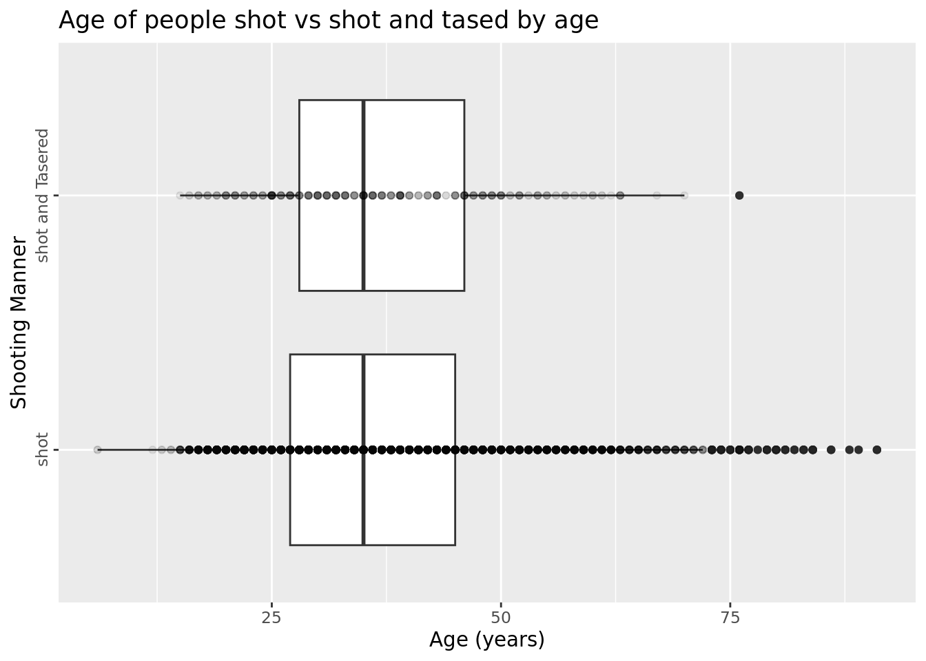
We plan to represent our four variables through a series of six graphics. Our preliminary graph will be a box plot to compare the ages of those shot vs shot and tasered. We will facet by shot/shot tasered, and our axis values will be age. This will help create a baseline understanding of what ages are most vulnerable to more violence. Having this knowledge will add significance to the future graphs that incorperate gender and race.
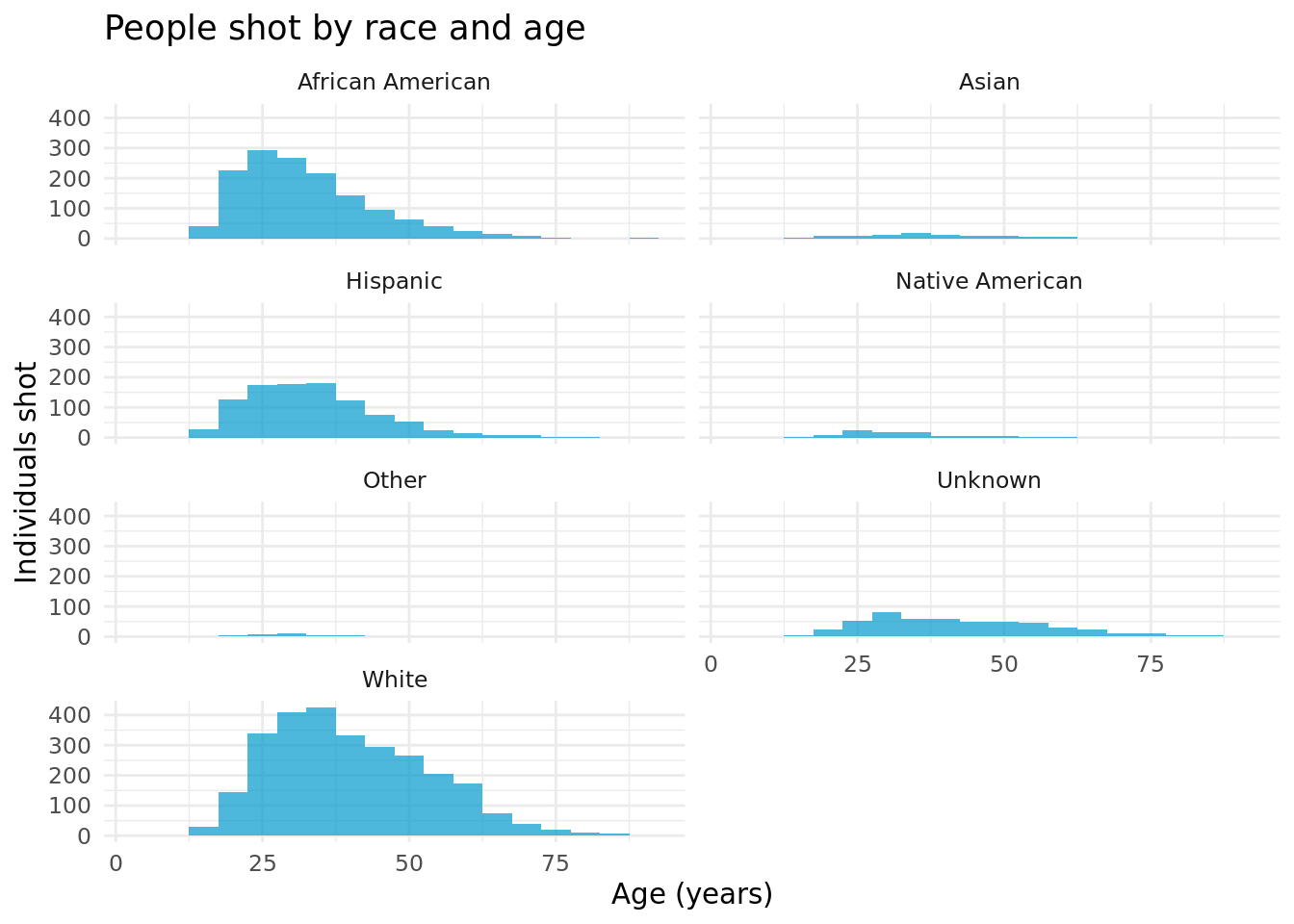
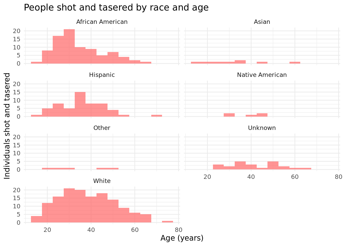
Our next two graphs will compare age, race, and shot/shot tasered. We will create one histogram faceted by race and filled by age, filtered for those only shot. Our next graph will be the same, except filtered for those shot and tasered; this will help visualize how age differs by race between those just shot and those shot and tasered.
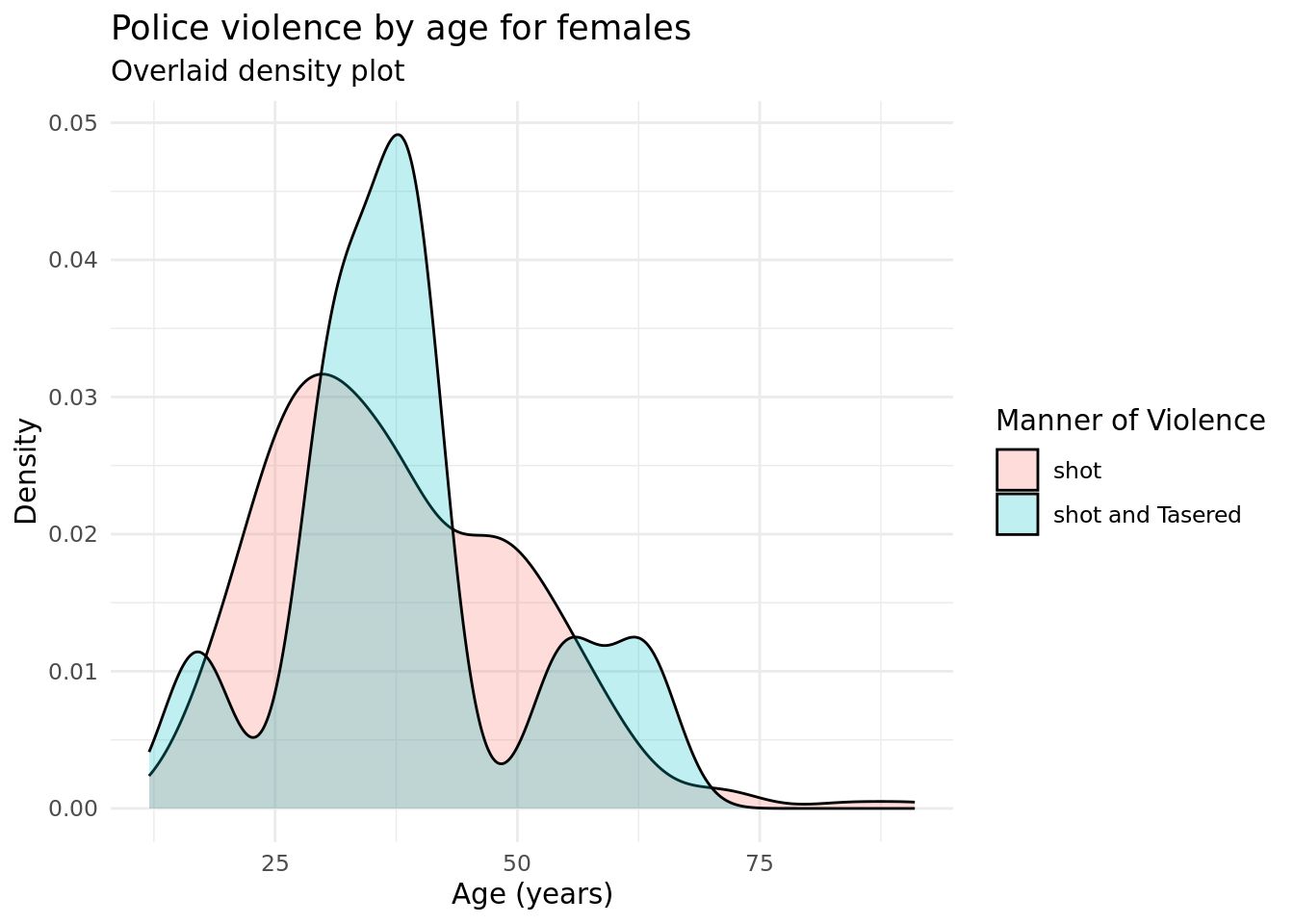
Next, we will create two overlaid density plots to compare age, gender, and shot/shot tasered. The first will be for females and put age on the x-axis and density on the y-axis, overlaying the graphs for shot and shot and Tasered. The second will be the same method, except using a graph filtered for males. These two graphs have a similar purpose to graphs 2 and 3, except they will be examining the affect of gender on level of violence instead of race.
Finally, we will include a graph of our additional variable, if the victim was fleeing or not (and how so). We predict that this variable might have an impact on if the victim was shot or shot and tasered, so we think it is important to include a representation of it. We will use a histogram with the three possibilities for fleeing on the x-axis (not fleeing, car, foot), and we will fill the graph by shot or shot and tasered. When making equations to analyze our data, we can use multiple linear regression analysis to estimate the importance and relevance of the extra explanatory variable (fleeing) and the response variable (level of violence). This helps account for fleeing status as a potentially confounding variable.
Based on the results, the model with the lowest AIC of one additional variable is age. Once examining the effects of gender, race and age on shooting manner independently of one another, we conclude the most prominent factors related to the violence level are age, followed by gender, and then race. Between the additive models, age and gender had a lower AIC than age and race, and the addition of all three variables had the highest AIC. The result is still worth exploring further through graphics. In the interactive models, age and gender also had a lower AIC than age and race. This means we may want to further investigate the correlation between age and gender in predicting shooting manner. For our purposes, we also decided to examine the effect of race on the severity of violence, as many current systemic issues in policing involve race. However, this round of AIC testing gave us a baseline understanding that in this data set, age is the most prominent predictor of shooting manner followed by gender.
Age, shot vs age, shot and tasered
Hypothesis test
\(H_o\): \(\mu_1 = \mu_2\) The mean age for people shot vs shot and tasered is equal.
\(H_a\) : \(\mu_1 \neq \mu_2\) The mean age for people shot and tasered is different than the mean age for shot alone.
# A tibble: 2 × 2
  Shooting.Manner  mean_age
  <chr>               <dbl>
1 shot                 37.1
2 shot and Tasered     36.9
The probability of observing a difference in means of 0.2757 years or more extreme between people shot and tasered vs shot alone, given the null assumption that the true difference in means is 0 years between groups, is 0.357. Therefore, we fail to reject the null hypothesis under the significance level alpha = 0.05 and conclude that there is weak evidence to support the alternative hypothesis.
Age, race, shot
# A tibble: 7 × 2
  Person.Race      mean_age
  <chr>               <dbl>
1 African American     32.6
2 Asian                36.8
3 Hispanic             33.6
4 Native American      31.9
5 Other                32.4
6 Unknown              42.4
7 White                40.1
# A tibble: 1 × 1
  mean_age
     <dbl>
1     34.6
Age, race, shot and tasered
# A tibble: 7 × 2
  Person.Race      mean_age
  <chr>               <dbl>
1 African American     34.5
2 Asian                33.8
3 Hispanic             35.7
4 Native American      37.6
5 Other                34
6 Unknown              41.1
7 White                38.3
Hypothesis test \(H_o\): \(\mu_1 = \mu_2\) The mean age for females shot vs shot and tasered is equal. \(H_a\) : \(\mu_1 \neq \mu_2\) The mean age for females shot and tasered is different than the mean age for shot alone.
# A tibble: 2 × 2
  Shooting.Manner  mean_age
  <chr>               <dbl>
1 shot                 37.4
2 shot and Tasered     38.4
The probability of observing a difference in means of 0.97 years or more extreme between females shot and tasered vs shot alone, given the null assumption that the true difference in means is 0 years between groups, is 0.396. Therefore, we fail to reject the null hypothesis under the significance level alpha = 0.05 and conclude that there is weak evidence to support the alternative hypothesis.
Age and shot/shot tasered (male)
Hypothesis test \(H_o\): \(\mu_1 = \mu_2\) The mean age for males shot vs shot and tasered is equal. \(H_a\) : \(\mu_1 \neq \mu_2\) The mean age for males shot and tasered is different than the mean age for shot alone.
# A tibble: 2 × 2
  Shooting.Manner  mean_age
  <chr>               <dbl>
1 shot                 37.1
2 shot and Tasered     36.8
The probability of observing a difference in means of 0.69725 years or more extreme between males shot and tasered vs shot alone, given the null assumption that the true difference in means is 0 years between groups, is 0.459 Therefore, we fail to reject the null hypothesis under the significance level alpha = 0.05 and conclude that there is weak evidence to support the alternative hypothesis.
We predict that younger age ranges will experience higher rates of violence (shot and tasered vs shot). People in the age range of young adult to mid-thirties (approximately 20 - 35) will experience higher rates of shot and tasered vs just shot. (graph 1)
(prediction for comparing 2 and 3) We predict that Hispanic and African-American targets will be shot and tased comparatively more than just shot; oppositely, white and Asian targets will be shot comparatively more than shot and tased.
(prediction for comparing 4 and 5) We predict that male gender targets will be shot and tased comparatively more than just shot; oppositely, female gender targets will be shot comparatively more than shot and tased.
When making a visualization of fleeing status vs. shot/shot and tased, we infer that the victim’s fleeing status affects the level of violence. We predict that those not fleeing will be shot and tased at the highest rate compared to just shot (because they’re in close proximity to tase), followed by fleeing on foot, and finally fleeing with a car. This prediction is based on how convenient and easy it is to tase and shoot compared to just shooting.
3. Results
Graph 1: This graph relates age to the shooting manner in which the individual was targeted (shot and tased vs shot alone). For both groups, the average age at which they were targeted was between ages 25-40, and it initially appears from the data visualization that age did not differ significantly between the groups of people shot and tasered vs shot alone. This was confirmed with hypothesis testing. Summary statistics were calculated for both shot and tasered (\(\mu\) = 36.08) and shot alone (\(\mu\) = 35.35) groups, and a p-value of 0.214 was calculated given the null hypothesis that the difference in means between groups was 0 years. As a result, we fail to reject the null hypothesis and conclude weak evidence for the alternative hypothesis that age significantly differs between groups.
Graphs 2 and 3: These two graphs shows the effect of race and age on violence severity at the hands of police. The trend across the first graph of those only shot was that the most likely age range to be shot for all demographics is from the mid twenties to late thirties. Specifically, the mean age to be shot by the police for white people is 40.05 years old, while the mean age to be shot for non-white BIPOC is 34.56 years old. This matched with our predictions. The races with the highest count of those shot were the African American, White, and Hispanic populations. We assumed that those of minority populations would be among the most targeted, and the data partially represents that hypothesis. The third graph shows the effect of race and age on victims who were both shot and tasered. Specifically, the mean age to be shot and tased by the police for white people is 38.32 years old, while the mean age to be shot and tased for non-white BIPOC is 35.71 years old. Again the trends center on those in the African American, Hispanic, and White populations, however the age spread is wider and older than the graphs of those who were only shot. Contrary to our assumptions, this seems to indicate that those shot and tasered span victims ages twenty to fifty in all races. We can conclude that there is no definitive correlation between age and whether or not someone was shot, or shot and tasered by age and race. However, there were peaks in the graph in victims of African American descent in their late twenties and early thirties, as well as white and Hispanic victims in their thirties. The majority of those shot and tasered were in their twenties to thirties and African American, Hispanic, and white races. However, this is very similar to the trend among those who were shot and not tasered, and there is no definitive effect that race and age has on the police officer’s shooting manner, whether they shoot or tase and shoot.
Graph 4: This graph is showing the overlaid density plot for females, comparing both shot and shot and Tasered. As we can see from the density plot, there seems to be three hotspots at which females experience more violence (shot and Tasered), around ages 10, 37, and 60. However, based on the hypothesis testing, there does not appear to be sufficient evidence that the mean age is really any different across the two categories. So, overall, the mean age at which people encounter the different types of violence does not appear to have any significant difference, but at certain ages, there does appear to be a greater or lesser probability to experience one type of violence over another.
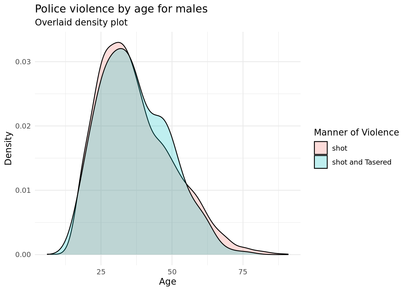
Graph 5: Compared to the graph for females, the male graph is almost indistinguishable when comparing shot and shot and Tasered. This seems to suggest that at least for males, whether or not they were tasered in addition to being shot did not really matter. Thus, the hypothesis that males will experience more violence (shot and Tasered) at younger ages seems to be disproven. This matches with our hypothesis testing which gave insufficient evidence to reject the null hypothesis (that mean age does not differ across categories).
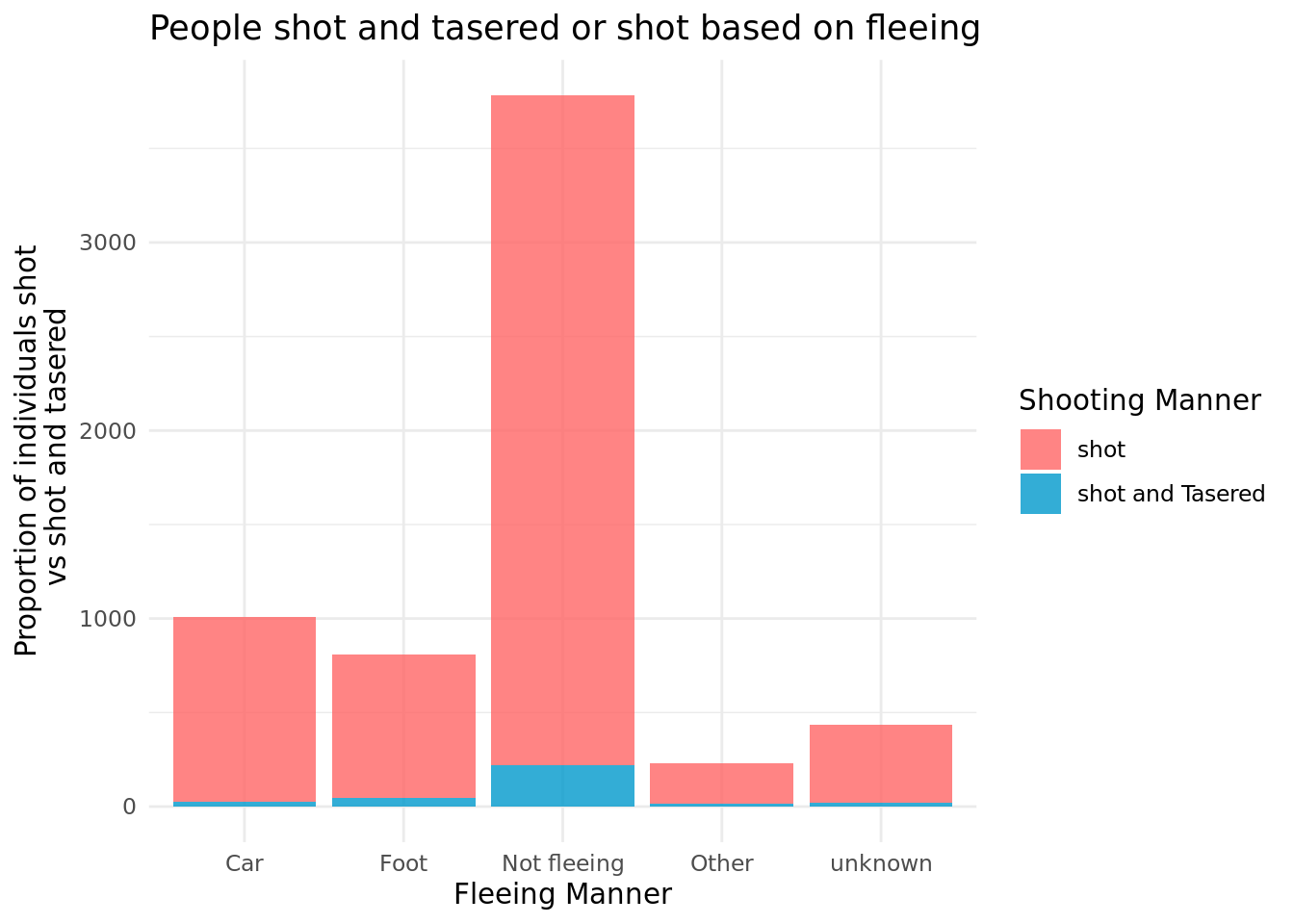
Graph 6: This graph shows the relationship between fleeing manner and whether or not someone was shot, or shot and tasered. Overall, there is little correlation between these two variables. Judging from the graph, it appears that the largest count of victims that were shot and tasered were not fleeing, followed by victims that were fleeing on foot. Proportionally, however, it does not appear that there is a correlation. Given that this analysis does not relate to our central hypothesis on race, age, gender, and severity of violence, we do not utilize forward selection or hypothesis testing. However, given our initial visualization, we do not think there is a large enough correlation to relate shooting manner and fleeing manner.
Discussion
Our overarching goal was to find how race and gender impact the average age of victims of police violence, and if those factors affect the level of violence they experience - shot vs shot and tasered. Overall, we concluded that age itself is relatively consistent between levels of violence, but minority groups experience both types of violence at younger ages (32 for African Americans, 36 for Asians, 33 for Hispanics, 31 for Native Americans) than white people (40). Gender also plays a role in the age, and type of violence that perpetrators experience. The mean probability of getting shot vs shot and tasered for males differs less by age than it does for females, but males in general experience more police violence (shot and tasered compared to just shot). Our findings confirm our hypothesis that minorities and men experience police violence at a higher rate, but we were wrong in predicting that younger people of minority races and both genders would be shot and tasered more than just shot - hypothesis tests showed that age for each race and gender did not determine level of violence. For graph number 6 in analyzing the relationship between fleeing manner and severity of violence, we could have improved our analysis by including a forward selection process for each fleeing manner in car, foot, not fleeing, other, or unknown. In the future, we would further investigate this relationship using a logistical regression.
Potential limitations of our analysis is prioritizing interactions between age and race/gender instead of also looking at the interactions between gender and race separately. Additionally, there is significantly more data on men than women so to truly get an understanding of how gender predicts level of violence it would be helpful to use a dataset with more comprehensive data on victims that were women. Finally, we analyzed level of violence by comparing shot to shot and tasered, but it would make sense to also compare these findings to police stoppages with no violence and interactions that end in harm or death. In the future we would be interested to include more detailed ways of tracking police violence (such as including police weapons used or time-of-encounter variables). Additionally, future work could look at what strategies can be taken to limit violence based on what measures have been successful in the past.