Logistic Regression

Lecture 16

Dr. Elijah Meyer

Duke University
STA 199 - Spring 2023

March 8th, 2022

Checklist

– Clone ae-15

Announcements

– HW 3 due Friday (3-10)

– Project Proposal due Friday (3-10)

Announcements: HW 6 - Statistics Experience

– The goal of the statistics experience assignments is to help you engage with the statistics and data science communities outside of the classroom

– No GitHub repo for this assignment

Experience statistics outside of the classroom

Examples

– Attend a talk or conference

– Talk with a statistician/ data scientist (myself and TAs do not count)

– Listen to a podcast / watch video

– Participate in a data science competition or challenge

– Read a book on statistics/data science

– TidyTuesday challenges

– Coding out loud project

Data Fest 2023 at Duke

– data analysis competition where teams of up to five students attack a large, complex, and surprise dataset over a weekend

– DataFest is a great opportunity to gain experience that employers are looking for

– Each team will give a brief presentation of their findings that will be judged by a panel of judges comprised of faculty and professionals from a variety of fields.

Hw 6 - Statistical Experience

– Summarize your experience

– Guidelines are in the instructions

Where is the assignment?

Warm Up

– What is the difference between R-squared and Adjusted R-squared?

— How are each defined?

— When are each appropriate to use?

Warm Up

– How are each defined?

R-squared: The proportion of variability in our response that is explained by our model

Adjusted-R-squared: Measure of overall model fit

Warm Up

— When are each appropriate to use?

R-squared: when the models have the same number of variables

Adjusted-R-squared: when the models have a different number of variables

Goals

– The What, Why, and How of Logistic Regression

What is Logistic Regreesion

• Similar to linear regression…. but

• Modeling tool when our response is categorical

What we will do today

– This type of model is called a generalized linear model

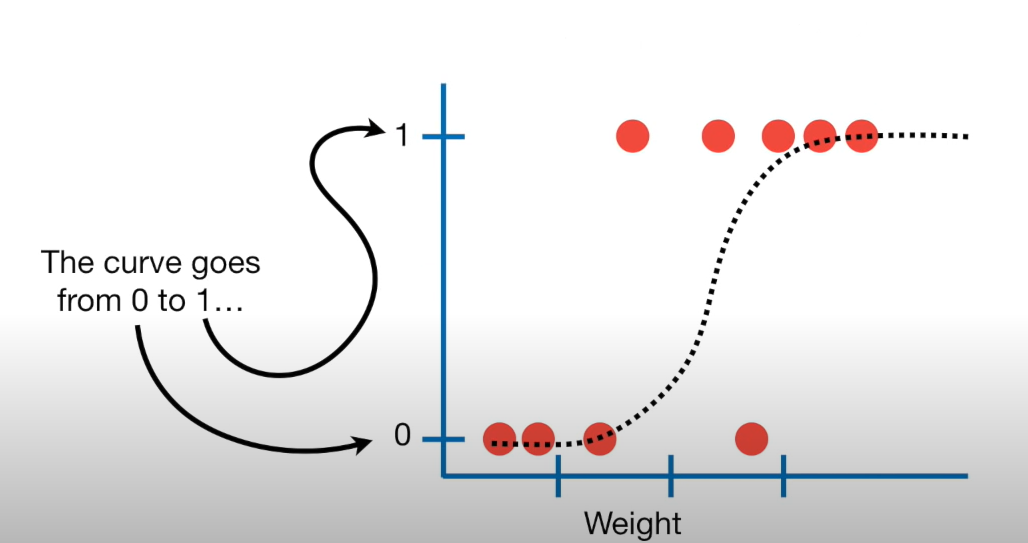
Start from the beginning

Terms

– Bernoulli Distribution

• 2 outcomes: Success (p) or Failure (1-p)

• \(y_i\) ~ Bern(p)

• What we can do is we can use our explanatory variable(s) to model p

2 Steps

– 1: Define a linear model

– 2: Define a link function

A linear model

\(\eta_i = \beta_o + \beta_1*X_i + ...\)

Note: We use \(p_i\) for estimated probabilities

• But we can’t stop here

Think about what a linear model looks like

Next steps

– Preform a transformation to our response variable so it has the appropriate range of values

Generalized linear model

• Next, we need a link function that relates the linear model to the parameter of the outcome distribution i.e. transform the linear model to have an appropriate range

Goal

– Or…. takes values between negative and positive infinity and map them to probabilities

Logit Link function

– A logit link function transforms the probabilities of the levels of a categorical response variable to a continuous scale that is unbounded

– Note: log is in reference to natural log

What’s this look like

Takes a [0,1] probability and maps it to log odds (-\(\infty\) to \(\infty\).)

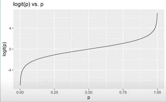
Almost….

This isn’t exactly what we need though…..

Will help us get to our goal

Logit Link Function

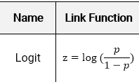
The logit link function is defined as follows:

Generalized linear model

• \(logit(p)\) = \(\widehat{\beta_o} +\widehat{\beta}_1X1 + ....\)

• logit(p) is also known as the log-odds

• logit(p) = \(log(\frac{p}{1-p})\)

• \(log(\frac{p}{1-p})\) = \(\widehat{\beta_o} +\widehat{\beta}_1X1 + ....\)

One final fix

– Recall, the goal is to take values between -\(\infty\) and \(\infty\) and map them to probabilities. We need the opposite of the link function… or the inverse

– How do we take the inverse of a natural log?

• Taking the inverse of the logit function will map arbitrary real values back to the range [0, 1]

So

• \(logit(p)\) = \(\widehat{\beta_o} +\widehat{\beta}_1X1 + ....\)

• \[log(\frac{p}{1-p}) = \widehat{\beta_o} +\widehat{\beta}_1X1 + ....\]

• Lets take the inverse of the logit function

\[p = \frac{e^{\widehat{\beta_o} + \widehat{\beta_1}X1 + ...}}{1 + e^{\widehat{\beta_o} + \widehat{\beta_1}X1 + ...}}\]

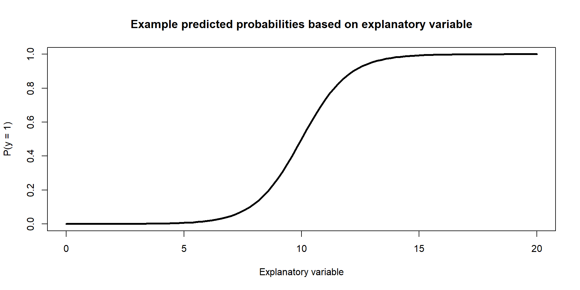
Example Figure:

What we will do today

ae-15

Takeaways

– We can not model these data using the tools we currently have

– We can overcome some of the shortcoming of regression by fitting a generalized linear regression model

– We can model binary data using an inverse logit function to model probabilities of success