Models + SLR
Lecture 12
Dr. Elijah Meyer
Duke University
STA 199 - Spring 2023
Feburary 22nd, 2023
Checklist
– Clone ae-11
Announcements
– HW-2 Due Friday at 11:59
– Lab 4 Due Tuesday at 11:59
Data Fest 2023 at Duke
– data analysis competition where teams of up to five students attack a large, complex, and surprise dataset over a weekend
– DataFest is a great opportunity to gain experience that employers are looking for
– Each team will give a brief presentation of their findings that will be judged by a panel of judges comprised of faculty and professionals from a variety of fields.

Lab 4
– Team Submission
– Attach ALL team members to submission on Gradescope
– Communicate!
– “It was my responsibility to turn the lab in and I forgot….”
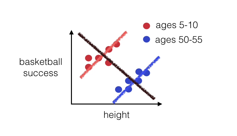
Warm up: Simpson’s Paradox
What is it?
Why is it important?
Warm up
Where we are going
\(\checkmark\) Data Viz
\(\checkmark\) Probability
– Modeling Data
Goals
– Introduce the idea of modeling
– Why we model data?
— Modeling with single predictors
— How to write equations
— Interpret Slopes
— Interpret Intercepts
Warm up 2
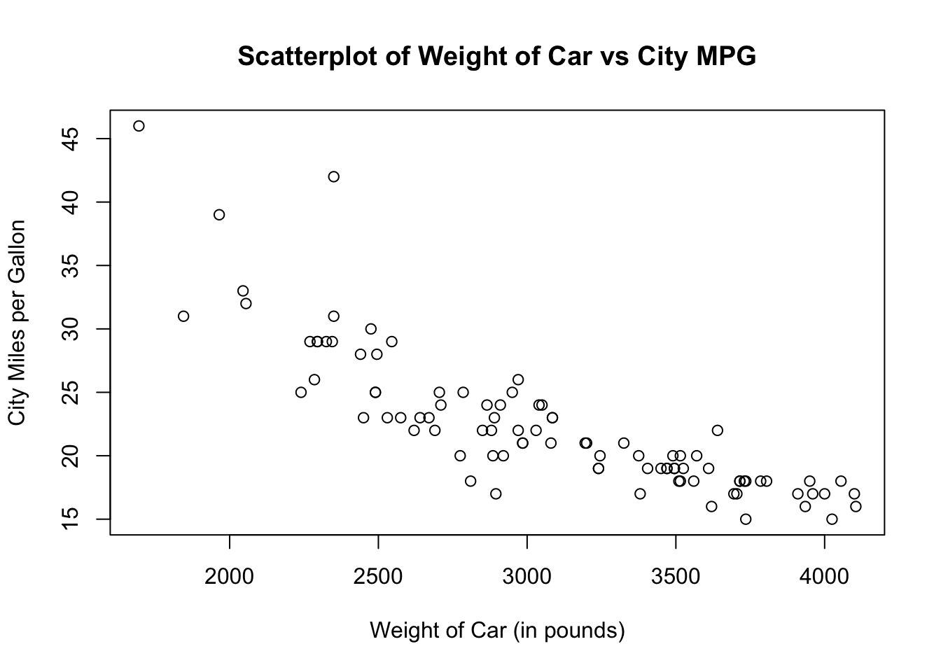
– What is the relationship?
– What is your best guess for a car’s MPG that weighs 5000 pounds? 3000 pounds?
What is a statistical model?
– Statistical modeling is the process of applying statistical analysis to a data set.
– A statistical model is a mathematical representation of observed data.
Why
– Interpretation
– Prediction
What is linear regression?
– Model data using a straight line
– Quantitative response
– Quantitative or categorical explanatory
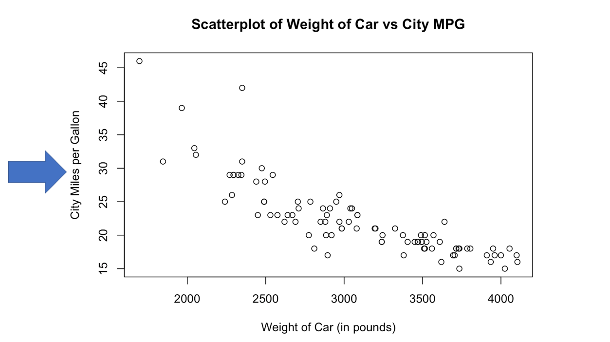
Vocab - Response variable
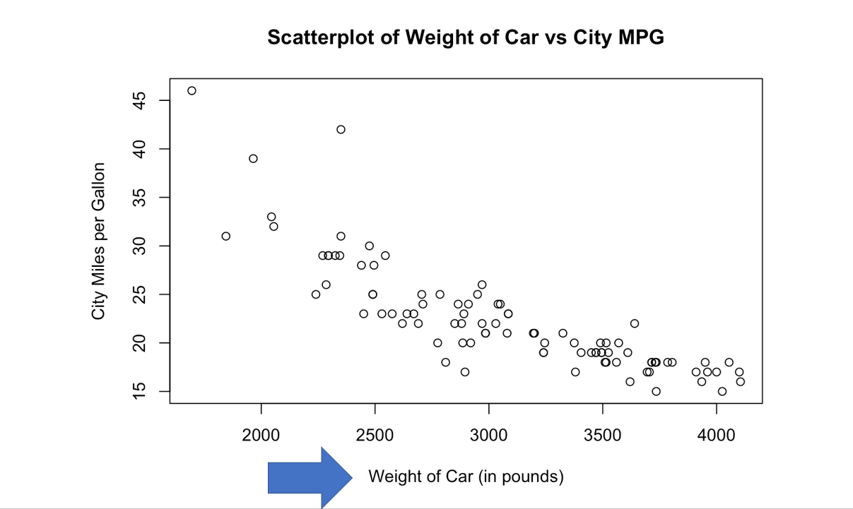
Vocab - Explanatory variable
How are Models Fit?

How are Models Fit?
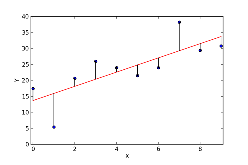
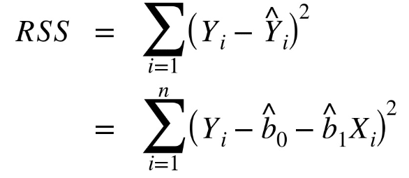
How are Models Fit?
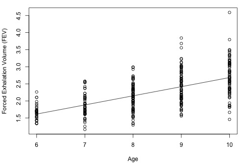
What about when X is categorical?
What about when X is categorical?
In R: SLR
linear_reg() |>

     set_engine("lm") |>

     fit(y ~ x , data = data-set ) |>

     tidy()
ae-11
Model Notation - Population
\[ Y_i = \beta\_o + \beta\_1x_i +\epsilon\_i\]
\[ Y\; - True\; mean\;response \]
\[\beta\_o\; -True\; intercept\]
\[\beta\_1\; - True\; slope\; coefficient\]
\[\epsilon\_i\; - Error\; term\; for\; each\; observation\; i\]
Model Notation - Estimated
\[\hat{Y} = b + b_1x\]
\[\hat{Y} = \hat{\beta_o} + \hat{\beta_1}x\]
\[\hat{Y} - estimated\; (predicted)\; mean \;response\]
\[\hat{\beta_o} - estimated\; intercept\]
\[\hat{\beta_1} - estimated\; slope\] We assume that our error term is normally distributed and has a mean of 0. Thus, it does not show up in our model.
Model Notes
Things to note:
X is our explanatory variable and is not random. We know the value of X.
Y is our response variable. For a fixed X, Y will be a random variable (have a random outcome).
This random outcome is observed based on a random draw from a distribution we assume.
When using this model for prediction, we expect Y to take on the most likely value for a given X… which is the center of the distribution.
Let’s draw it out…
Takeaway
So, for an observed X….. we are modeling the mean of the distribution of Y
Or, Y is a mean response
“we estimate a mean change in Y”
“we estimate, on average…..”
This is extremely important when we think about interpretation
Summary
– Y is a random variable.
– We assume that observations from this random variable are normally distributed.
– Because of this distributional assumption, we are modeling the mean of Y and not just Y.
Wrap up: Check yourself
– What is a model?
– What are the 2 main reasons we fit models?
– Slope coefficients? Intercepts?
– How does linear regression change when x is quantitative vs categorical?
