Rows: 50
Columns: 1
$ ppg <dbl> 48.00000, 40.00000, 99.00000, 13.00000, 55.00000, 75.00000, 74.000…Suggested Answers: AE-20
Hypothesis Testing
Learning goals
By the end of today, you will…
- Use simulation-based methods to test a claim about a population parameter
- Use simulation-based methods to generate the null distribution
- Calculate and interpret the p-value
- Use the p-value to draw conclusions in the context of the data
We have data on the price per guest (ppg) for a random sample of 50 Airbnb listings in 2020 for Asheville, NC. We are going to use these data to investigate what we would of expected to pay for an Airbnb in in Asheville, NC in June 2020. Read in the data and answer the following questions. Today, we are going to investigate if the mean price of an Airbnb in Ashville, NC in June 2020 was larger than 60.
Setting up the hypotheses
Based on the context of the problem, write out the correct null and alternative hypothesis. Do this in both words and in proper notation.
\(H_o: \mu = 60\)
\(H_a: \mu > 60\)
The true (population) mean price per guest of airbnbs in NC 2020 is equal to $60
The true (population) mean price per guest of airbnbs in NC 2020 is larger than $60
Motivation
We want to know how unlikely it would be to observe our statistic under the assumption of the null hypothesis. Calculate and report the sample statistic below using proper notation.
\(\bar{x}\) = 76.6
Building a distribution
Let’s use simulation-based methods to conduct the hypothesis test specified above. We’ll start by generating the null distribution.
- How do we generate the null distribution? Detail the steps below.
Subtract 16.6 from each of of 50 observations
Next….
Sample with replacement 50 times
Calculate the new resampled mean
This resampled mean is one “dot” or one observation
Repeat the process above many many times
Let’s repeat this process many many times below
set.seed(101321)

library(tidymodels)
── Attaching packages ────────────────────────────────────── tidymodels 1.0.0 ──✔ broom 1.0.1 ✔ rsample 1.1.0
✔ dials 1.1.0 ✔ tune 1.0.1
✔ infer 1.0.3 ✔ workflows 1.1.0
✔ modeldata 1.0.1 ✔ workflowsets 1.0.0
✔ parsnip 1.0.3 ✔ yardstick 1.1.0
✔ recipes 1.0.3 Warning: package 'broom' was built under R version 4.2.2Warning: package 'dials' was built under R version 4.2.2Warning: package 'parsnip' was built under R version 4.2.2Warning: package 'recipes' was built under R version 4.2.2── Conflicts ───────────────────────────────────────── tidymodels_conflicts() ──
✖ scales::discard() masks purrr::discard()
✖ dplyr::filter() masks stats::filter()
✖ recipes::fixed() masks stringr::fixed()
✖ dplyr::lag() masks stats::lag()
✖ yardstick::spec() masks readr::spec()
✖ recipes::step() masks stats::step()
• Learn how to get started at https://www.tidymodels.org/start/null_dist <- abb |>
specify(response = ppg) |>
hypothesize(null = "point", mu = 60) |>
generate(reps = 1000, type = "bootstrap") |>
calculate(stat = "mean")Take a glimpse at null_dist. What does this represent?
glimpse(null_dist)Rows: 1,000
Columns: 2
$ replicate <int> 1, 2, 3, 4, 5, 6, 7, 8, 9, 10, 11, 12, 13, 14, 15, 16, 17, 1…
$ stat <dbl> 54.94833, 60.20833, 48.79833, 55.28833, 64.59000, 42.30500, …Visualize
Now, create an appropriate visualization fo your null distribution. Where is this distribution centered? Why does this make sense?
null_dist |>
  ggplot(
    aes(x = stat)
  ) +
  geom_histogram()
`stat_bin()` using `bins = 30`. Pick better value with `binwidth`.
60 and this makes sense We assume the true mean ppg is equal to 60. Data were shifted and resampled from, meaning that we would expect this distribution to be centered at 60.
Now, add a vertical line on your null distribution that represents your sample statistic. Based on the position of this line, do you your sample mean is an unusual observation under the assumption of the null hypothesis?
null_dist |>
  ggplot(
    aes(x = stat)
  ) +
  geom_histogram() +
  geom_vline(xintercept = 76.6)
`stat_bin()` using `bins = 30`. Pick better value with `binwidth`.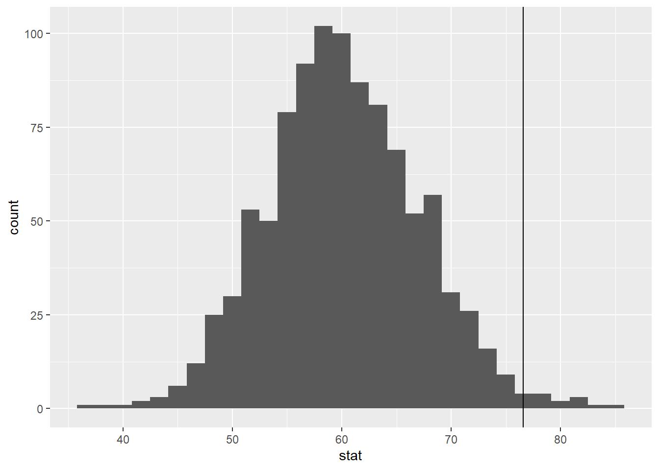
Let’s quantify your answer above….
p-value
What is a p-value?
Probability of observing our sample statistic, “or something more extreme” given the null hypothesis is true.
or more extreme is in reference to Ha
How can we calculate it? Things to consider….
We need to know our statistic
We need to recall the sign of the alternative hypothesis
Let’s put this in motion!
We are going to calculate the p-value in two different ways. The first one is “by-hand”
Let’s think about what’s happening when we run get_p_value. Fill in the code below to calculate the p-value “manually” using some of the dplyr functions we’ve learned.
- Calculate your p-value
# A tibble: 1 × 1
  p_value
    <dbl>
1 0.012- Calculate your p-value below
null_dist |>
  get_p_value(obs_stat = 76.6, direction = "greater")
# A tibble: 1 × 1
p_value
<dbl>
1 0.012Let’s visualize it!
visualize(null_dist) +
 shade_p_value(obs_stat = 76.6, direction = "greater")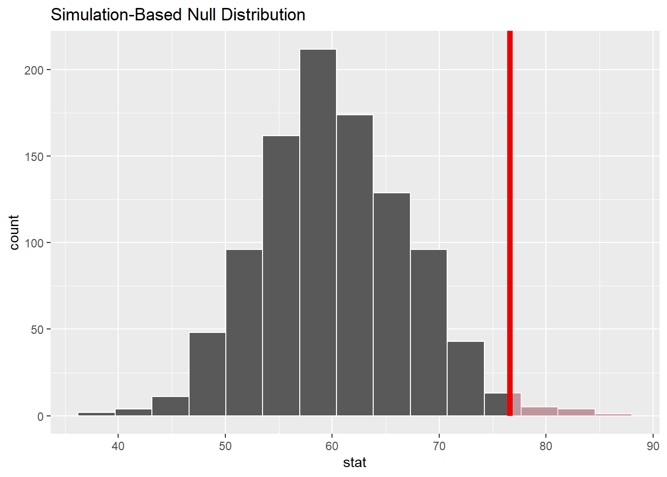
- Interpret your p-value in the context of the problem
Probability of observing our sample statistic, “or something more extreme” given the null hypothesis is true.
The probability of observing $76.6 or larger, given that true (population) mean price per guest of airbnbs in NC 2020 is equal to $60 is equal to ~ 0.012
Conclusion
Use the p-value to make your conclusion using a significance level of 0.05. Remember, the conclusion has 3 components
\(\alpha\) How much evidence we need to reject or fail to reject the null hypothesis
- How the p-value compares to the significance level
- The decision you make with respect to the hypotheses (reject \(H_0\) /fail to reject \(H_0\))
- The conclusion in the context of the alternative hypothesis
Significance level
What is it?
\(\alpha\) = a measure of the strength of the evidence that must be present in your sample before rejecting the null and concluding your alternative hypothesis
\(\alpha\) = 0.05 > p-value 0.012 Reject the null hypothesis (decision)
(conclusion) Strong evidence to conclude the alternative hypothesis
Example:
\(\alpha\) = 0.05 < p-value 0.120 Failing to reject our null hypothesis Weak evidence to conclude the alternative hypothesis
Two-sided
Suppose instead you wanted to test the claim that the mean price of an Airbnb is not equal to $60. Which of the following would change? Select all that apply.
- Null hypothesis b. Alternative hypothesis
- Null distribution d. p-value
Conclusion
Let’s test the claim in last exercise. Conduct the hypothesis test.
null_dist |>
  get_p_value(obs_stat = 76.6, direction = "two sided")
# A tibble: 1 × 1
p_value
<dbl>
1 0.024Optional
We can never conclude the null hypothesis…. but why?
Let’s assume your null hypothesis for the Airbnb question is: \(\mu\) = 70, and you are interested in \(\mu\) > 70
null_dist2 <- abb |>
  specify(response = ppg) |>
  hypothesize(null = "point", mu = 70) |>
  generate(reps = 1000, type = "bootstrap") |>
  calculate(stat = "mean")

visualize(null_dist2) +
 shade_p_value(obs_stat = 76.6, direction = "greater")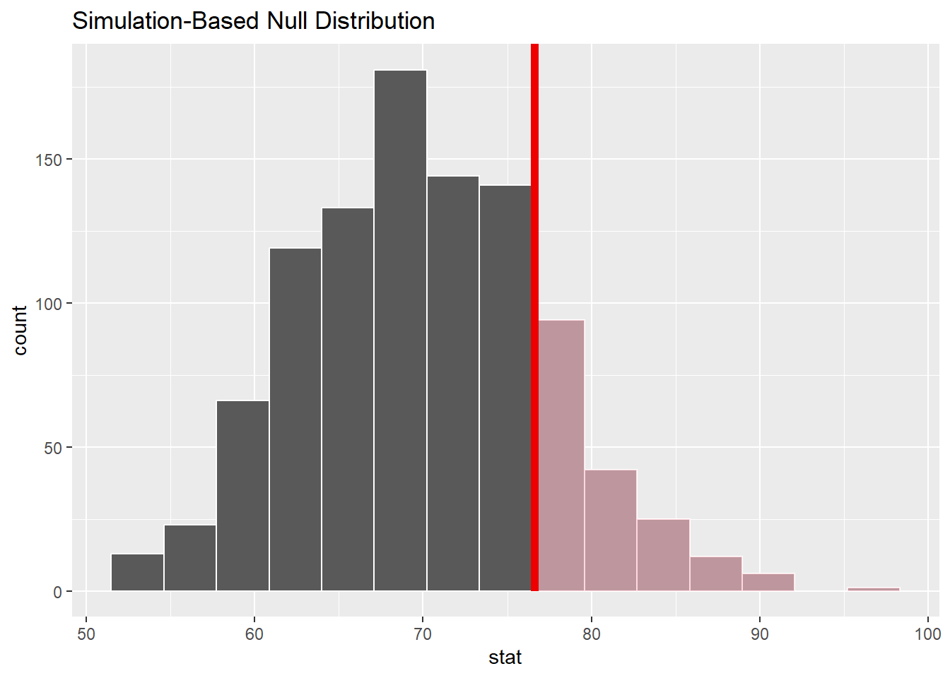
null_dist2 |>
  get_p_value(obs_stat = 76.6, direction = "greater")
# A tibble: 1 × 1
p_value
<dbl>
1 0.176So now…. I incorrectly conclude that \(\mu\) = 70.
Another research assumes that \(\mu\) = 72….
null_dist3 <- abb |>
  specify(response = ppg) |>
  hypothesize(null = "point", mu = 72) |>
  generate(reps = 1000, type = "bootstrap") |>
  calculate(stat = "mean")

visualize(null_dist3) +
 shade_p_value(obs_stat = 76.6, direction = "greater")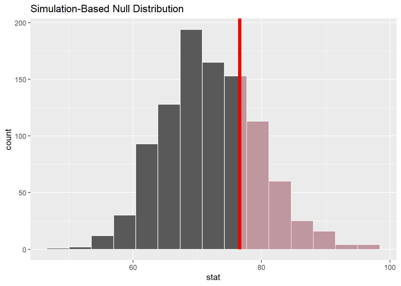
null_dist3 |>
  get_p_value(obs_stat = 76.6, direction = "greater")
# A tibble: 1 × 1
p_value
<dbl>
1 0.266So now…. I incorrectly conclude that \(\mu\) = 72….??????