Warning: package 'broom' was built under R version 4.2.2
Warning: package 'dials' was built under R version 4.2.2
Warning: package 'parsnip' was built under R version 4.2.2
Warning: package 'recipes' was built under R version 4.2.2
── Conflicts ───────────────────────────────────────── tidymodels_conflicts() ──
✖ scales::discard() masks purrr::discard()
✖ dplyr::filter()   masks stats::filter()
✖ recipes::fixed()  masks stringr::fixed()
✖ dplyr::lag()      masks stats::lag()
✖ yardstick::spec() masks readr::spec()
✖ recipes::step()   masks stats::step()
• Learn how to get started at https://www.tidymodels.org/start/
Load Data: Pokemon
We will be using the pokemon data set, which contains information about 42 randomly selected Pokemon (from all generations). Pokemon is a Japanese media franchise managed by The Pokémon Company, founded by Nintendo, Game Freak, and Creatures. Within this franchise, there are over 1000 different pokemon characters. In this activity, we are going to be taking estimating the mean height of them all.
You may load in the data set with the following code:
Rows: 42 Columns: 15
── Column specification ────────────────────────────────────────────────────────
Delimiter: ","
chr  (4): name, leg_status, type_1, type_2
dbl (11): pokedex_number, generation, height_m, weight_kg, bst, hp, atk, def...

ℹ Use `spec()` to retrieve the full column specification for this data.
ℹ Specify the column types or set `show_col_types = FALSE` to quiet this message.
In this analysis, we will use CLT-based inference to draw conclusions about the mean height among all Pokemon species.
EDA
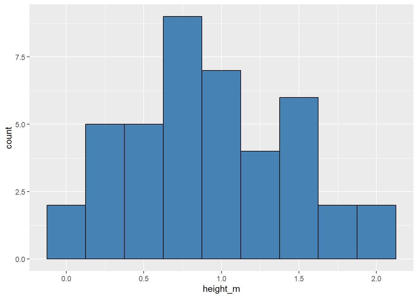
Let’s start by looking at the distribution of height_m, the typical height in meters for a Pokemon species, using a visualization and summary statistics.
pokemon|>ggplot(aes(x =height_m))+geom_histogram(binwidth =.25, fill ="steelblue", color ="black")
Below, calculate the mean, standard deviation, and sample size below…
Now, we will start on using the Central Limit Theorem to draw conclusions about the \(\mu\), the mean height in the population of Pokemon.
What is the point estimate for \(\mu\), i.e., the “best guess” for the mean height of all Pokemon? Use proper notation.
What is the point estimate for \(\sigma\), i.e., the “best guess” for the standard deviation of the distribution of Pokemon heights? Use proper notation.
CLT Conditions
Before moving forward, let’s check the conditions required to apply the Central Limit Theorem. Are the following conditions met:
Independence?
We have no reason to believe this is violated, as we took a random sample
Sample size?
Yes, we have a sample size larger than 30
Central limit theorem
Remember, when the independence and sample size assumptions are met, the central limit theorem states
\[
\bar{x} \sim N(\mu, \sigma / \sqrt{n})
\]
If we know \(\sigma\), we can construct a symmetric confidence interval for the true mean easily using qnorm() (using a normal distribution).
For example, if the true standard deviation in pokemon height is 0.4 meters, then to construct a 95% confidence interval:
xbar<-pokemon|>summarize(xbar =mean(height_m))|>pull(xbar)qnorm(c(0.025, 0.975), mean =xbar, sd =0.4)
In general, the confidence interval can be written as
\[
\bar{x} \pm z^* \times SD(\bar{x})
\]
where \(z^*\) is the quantile of a standard normal distribution associated with our level of confidence and the \(SD(\bar{x})\) is \(\sigma / \sqrt{n})\)
In Practice
If \(\sigma\) is unknown, it is more appropriate to be using a t-distribution to account for this additional uncertainty. We estimate the standard deviation of our sample mean with the standard error: ()
Many researchers estimate \(\sigma_\bar{x}\) with () and still use qnorm() if our sample size is “large.” This is what we did in ae-18 and we will revisit it later in the activity.
Practical confidence intervals
We don’t know the true population mean \(\mu\) and standard deviation \(\sigma\), how do we use CLT to construct a confidence interval?
We approximate \(\mu\) by \(\bar{x}\) and \(\sigma\) by with \(s\). However \(s\) may be smaller than \(\sigma\) and our confidence interval could be too narrow, for example, run the code below to compute the standard deviation of three draws from a standard normal.
Run this code a few times to repeat the simulation; you will find that \(s\) is sometimes above and sometimes below the true standard deviation we have set to 0.40.
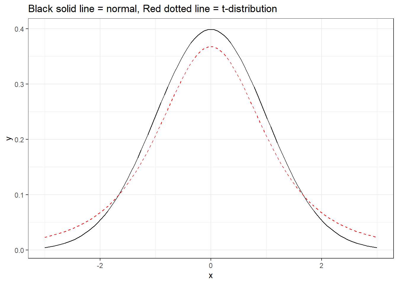
To account for this uncertainty, we will use a distribution with thicker tails. This sampling distribution is called a t-distribution.
ggplot(data =data.frame(x =c(0-1*3, 0+1*3)), aes(x =x))+stat_function(fun =dnorm, args =list(mean =0, sd =1), color ="black")+stat_function(fun =dt, args =list(df =3), color ="red",lty =2)+theme_bw()+labs(title ="Black solid line = normal, Red dotted line = t-distribution")
The t-distribution has a bell shape but the extra thick tails help us correct for the variability introduced by using \(s\) instead of \(\sigma\).
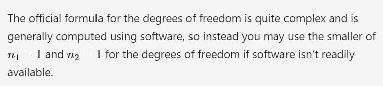
Unlike the normal distribution…. there are many many many different t-distributions. We can distinguish the differences by their degrees of freedom. The degrees of freedom describes the precise form of the bell-shaped t-distribution. In general, we’ll use a t-distribution with \(df=n−1\) to model the sample mean when the sample size is \(n\).
We can use qt and pt to find quantiles and probabilities respectively under the t-distribution.
Confidence interval
To construct our practical confidence interval (where we don’t know \(\sigma\)) we use the t-distribution:
In the last application exercise, we calculated a 95% confidence interval for true mean flipper length using a normal distribution (see code below). Let’s compare the results to a t-distribution…
They are the same because the sample size is large
Bootstrap for a difference in means
The Iris Dataset contains four features (length and width of sepals and petals) of 50 samples of three species of Iris (Iris setosa, Iris virginica and Iris versicolor). A sepal is the outer parts of the flower (often green and leaf-like) that enclose a developing bud. The petal are parts of a flower that are the pollen producing part of the flower that are often conspicuously colored. The difference between sepals and petals can be seen below.
The data were collected in 1936 at the Gaspé Peninsula, in Canada. For the first question of the exam, you will use this data sets to investigate a variety of relationships to learn more about each of these three flower species. The data set is prepackaged in R, and is called iris.
Goal: Previously, we have calculated confidence intervals for a single mean. Now, we are going to calculate confidence intervals for a difference in means.
Specifically, we are going to calculate the difference in mean Sepal length between the Setosa and Versicolor
EDA
First, we want to filter the data set to only contain our two Species. Please create a new data set that achieves this below.
# A tibble: 2 × 2
  Species    mean_l
  <fct>       <dbl>
1 setosa       5.01
2 versicolor   5.94
Central Limit Theorem or Bootstrap?
Are we justified to use the central limit theorem? Why or why not? Use code when able to justify your answer. For this activity, you can assume that these measurements come from a random sample.
Yes. These data come from a random sample and n is larger than 30 for each group
Suppose that the flowers did not come from a random sample. What are some ways that the independence assumption could be violated?
AWV. Think about spatial dependence or time dependence
Bootstrap
Regardless of your answer above, we are going to create a 90% confidence interval using bootstrap methods. Before we use R to generate this, let’s go over how this distribution is created.
How is one “dot” (observation) created on our bootstrap resampled distribution? Detail the steps below:
– Resample with replacement within each group 50 times.
– Calculate the new resampled means.
– Subtract the resampled means.
Bootstrap Confidence Interval
Similar to the last exercise… we will use bootstrapping to estimate the variability associated with the difference in sample means when taking repeated samples
boot_df<-iris_filter|>specify(response =Sepal.Length, explanatory =Species)|>generate(reps =1000, type ="bootstrap")|>calculate(stat ="diff in means")
Dropping unused factor levels virginica from the supplied explanatory variable 'Species'.
Warning: The statistic is based on a difference or ratio; by default, for
difference-based statistics, the explanatory variable is subtracted in the
order "setosa" - "versicolor", or divided in the order "setosa" / "versicolor"
for ratio-based statistics. To specify this order yourself, supply `order =
c("setosa", "versicolor")` to the calculate() function.
Now, let’s use boot_dfto create our 90% confidence interval.
Interpret your 90% confidence interval in the context of the problem below:
We are 90% confident that the true mean sepal length for setosa is 1.07 to 0.790 smaller than the true mean sepal length for versicolor
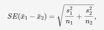
Note about theory based inference for difference in means….
Using theory based inference is almost identical to the single mean case. However, the standard deviation of our statistic uses both the standard deviation of the first and second group. See the following formula below…