Suggested Answers: CLT
Central Limit Theorem
To start this activity, we are going to demonstrate what the CLT is all about.
Below, we are going to generate a population distribution. This is not observed in real life. We are simply pretending we know this for demonstration purposes.
rs_pop <- tibble(x = rbeta(100000, 1, 5) * 100)


rs_pop |>
  ggplot(
    aes(x = x)) +
geom_density(fill = "blue") 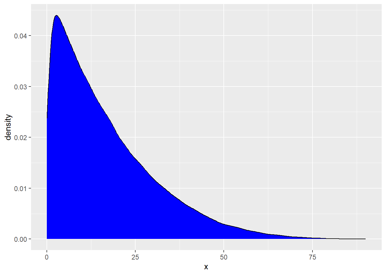
We are now going to draw samples from this population distribution, take the mean and repeat this process!
Below, draw one sample.
# A tibble: 1 × 1
  x_bar
  <dbl>
1  18.9
To make a distribution of sample means…. we need to do this process over and over and over again. Let’s do this below.
Now, create a histogram of the sample means below. But, before you do…. please answer the following question:
– Do you expect this distribution to be normally distributed or not? Justify your answer?
Yes! We meet the sample size requirement. n greater than 30
sampling |>
  ggplot(
    aes(x = xbar)
  ) +
  geom_histogram()
`stat_bin()` using `bins = 30`. Pick better value with `binwidth`.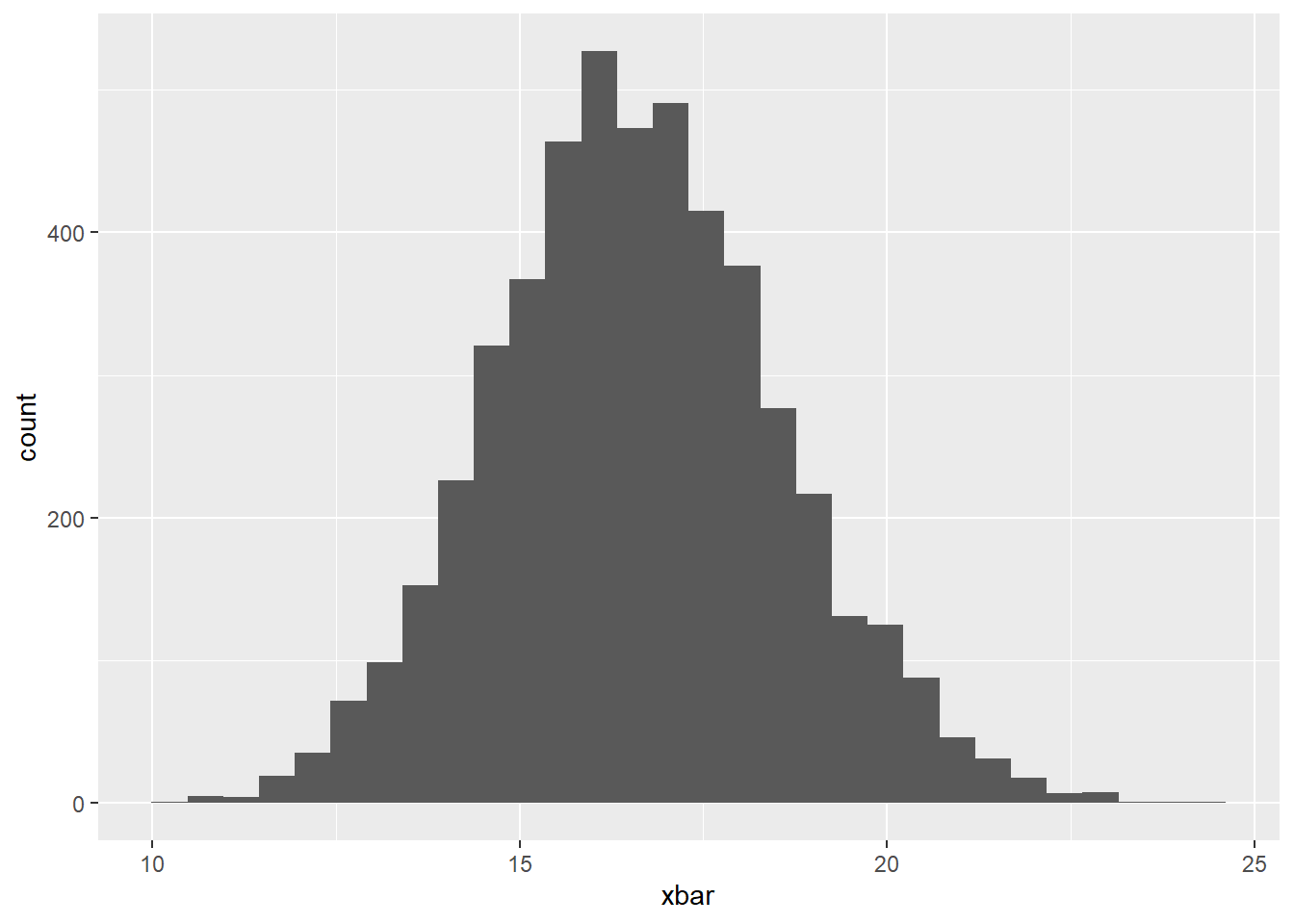
We know that the mean of our sampling distribution should be about the same as the mean of our population distribution. Check this below:
# A tibble: 1 × 1
      m
  <dbl>
1 16.6# A tibble: 1 × 1
m
<dbl>
1 16.6Takeaway And we can use this to create confidence intervals for our population parameter of interest (much like we can with bootstrap methods)
Small Sample Size
Now, let’s change our sample size to 3, violating as assumption of the CLT, and see how it impacts our sampling distribution.
Again, create a histogram of the sample means and comment on the shape of the distribution below.
sampling |>
  ggplot(
    aes(x = xbar)
  ) +
  geom_histogram()
`stat_bin()` using `bins = 30`. Pick better value with `binwidth`.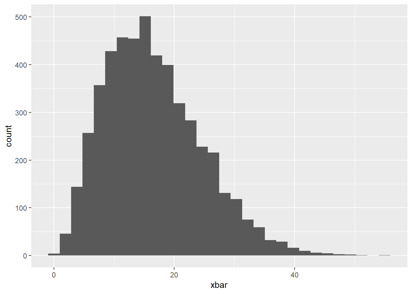
The histogram is skewed right
Central Limit Theorem vs Bootstrapping
Now, we will use each method to calculate 95% confidence intervals for true mean flipper length of penguins using each method.
Bootstrap Confidence Interval
penguins2 <- penguins |>
  filter(species !="Gentoo")

boot_df <- penguins2 |>
  specify(response = flipper_length_mm , explanatory = species) |>
  generate(reps = 20000, type = "bootstrap") |>
  calculate(stat = "diff in means")
Dropping unused factor levels Gentoo from the supplied explanatory variable 'species'.Warning: Removed 1 rows containing missing values.Warning: The statistic is based on a difference or ratio; by default, for
difference-based statistics, the explanatory variable is subtracted in the
order "Adelie" - "Chinstrap", or divided in the order "Adelie" / "Chinstrap"
for ratio-based statistics. To specify this order yourself, supply `order =
c("Adelie", "Chinstrap")` to the calculate() function.Now, let’s use boot_dfto create our 95% confidence interval.
# A tibble: 1 × 2
  lower upper
  <dbl> <dbl>
1 -7.86 -3.87
Interpret your 95% confidence interval in the context of the problem below:
We are 95% confident that the true mean flipper length for penguins is between 199 and 202 mm.
CLT
Are we justified to use CLT to create a 95% confidence interval? Why or why not?
Independence - We will assume this is a random sample of all penguins
Sample Size - 344 greater than 30
Fill in the following code to calculate a 95% CI using the CLT
# A tibble: 1 × 1
      m
  <dbl>
1  201.
est_mu <- 201
est_sigma <- sd(penguins$flipper_length_mm , na.rm = T) / sqrt(344)
qnorm(c(0.025, 0.975), est_mu, est_sigma)[1] 199.514 202.486Is the CI from CLT the same or different than the one using bootstrap methods?
The Same
BUT
These were only roughly the same because of a large sample size. With a small sample size, we need to use a distribution different from Normal. See AE-19!