Suggested Answers:Regression with a Categorical Single Predictor + MLR

Packages

library(tidyverse)
library(tidymodels)
library(palmerpenguins)

We will continue to study penguins as we become more familiar with SLR and MLR procedures.

Categorical Explanatory

A different researcher wants to look at body weight of penguins based on the island they were recorded on. What’s different between this question and the question from ae-11? Hint: Think about the variable type.

Categorical Explanatory Variable

Make a dot plot with species on the x-axis to investigate this relationship below. Additionally, calculate the mean body mass by island below.

penguins |>
  ggplot(
    aes(y = body_mass_g, x = island)
  ) + 
  geom_point()

Warning: Removed 2 rows containing missing values (`geom_point()`).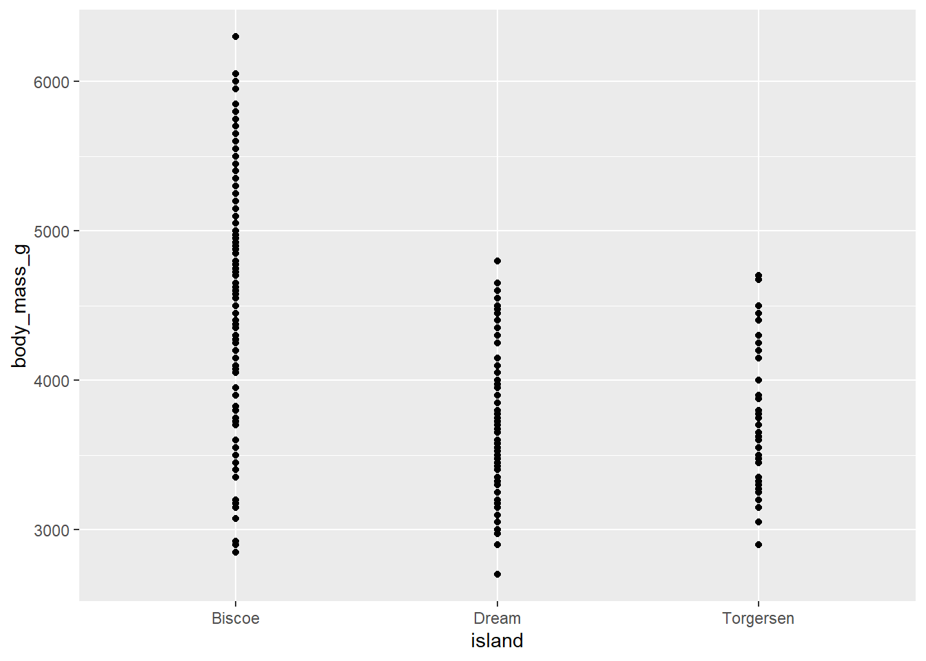

penguins |>
  group_by(island) |>
  summarize(mean_mass = mean(body_mass_g , na.rm = T))

# A tibble: 3 × 2
  island    mean_mass
  <fct>         <dbl>
1 Biscoe        4716.
2 Dream         3713.
3 Torgersen     3706.

Now, fit the linear regression model and display the results. Write the estimated model output below.

model2 <- linear_reg() |>
  set_engine("lm") |>
  fit(body_mass_g ~ island , data = penguins)

\(\widehat{body_mass_g} = 4716 - 1003*Dream - 1010*Torgersen\)

{1 if Dream; 0 if not} {1 if Torgersen; 0 if not}

Interpretation

What is the estimated mean body weight of a penguin on Dream island?

The estimated mean body weight of a penguin on Dream island is (4716 - 1003) grams.

How do we interpret this?

We estimate penguins on the dream island to weigh, on average 1003 grams less than those on the Bisoce island.

What is the estimated body weight of a penguin on Biscoe island? Where is it….?

Check the intercept!

Multiple Linear Regression

Additive model

In the last class, we modeled body mass by flipper length. Today, in a separate model, we modeled body mass by island. Could it be possible that the estimated body mass of a penguin changes by both their flipper length AND by the island they are on?

In multiple linear regression, we will discuss two different types of models. Additive models and interaction models. What’s the difference?

Additive models force the slopes to be the same across Z

Interaction models allow the slopes to be different

Now, fit an additive model to assess the relationship between our response variable body mass, and our explanatory variables flipper length and island. Produce the summary output. Write out the estimate regression equation below.

model1 <- linear_reg() |>
  set_engine("lm") |>
  fit(body_mass_g ~ flipper_length_mm , data = penguins) 


linear_reg() |>
  set_engine("lm") |>
  fit(body_mass_g ~ flipper_length_mm , data = penguins) |>
  tidy()

# A tibble: 2 × 5
  term              estimate std.error statistic   p.value
  <chr>                <dbl>     <dbl>     <dbl>     <dbl>
1 (Intercept)        -5781.     306.       -18.9 5.59e- 55
2 flipper_length_mm     49.7      1.52      32.7 4.37e-107

\(\widehat{body_mass_g} = -4625 + 44.5*flipper_length_mm - 262*Dream - 185*Torgersen\)

– Interpret the slope coefficient for flipper length in the context of the problem

“Holding all else constant”

Holding island constant (holding all other variables constant), for a one mm increase in flipper length, we estimate a 44.5 gram increase in mean body mass.

– Interpret the slope coefficient for Dream island in the context of the problem

Holding flipper length constant, we estimate the mean body mass of penguins on the dream island to be 262 grams less than those on the Bisoce island.

– Predict the body mass of a penguin with a flipper length of 200 on the Dream island

Hint: We can do this in R. Fill in the following code below:

Note: Name your model and do not pipe it into tidy() if you want to use the predict function

predict(model1, data.frame(flipper_length_mm = 200, island = "Dream"))

# A tibble: 1 × 1
  .pred
  <dbl>
1 4156.

R-squared

– What is R-squared?

R-squared is the percent variability in the response that is explained by our model. (Can use when models have same number of variables for model selection)

How can we calculate this in R?

glance(model1)$r.squared

[1] 0.7589925