Suggested Answers: Regression with a Single Predictor
Packages
Today, we will revisit the penguins data set. If needed, please re-familiarize yourself by reading the following context and taking a glimpse at the data set before we get started.
This data set comprising various measurements of three different penguin species, namely Adelie, Gentoo, and Chinstrap. The rigorous study was conducted in the islands of the Palmer Archipelago, Antarctica. These data were collected from 2007 to 2009 by Dr. Kristen Gorman with the Palmer Station Long Term Ecological Research Program, part of the US Long Term Ecological Research Network. The data set is called penguins.
- Take a glimpse of the data set below.
glimpse(penguins)Rows: 344
Columns: 8
$ species <fct> Adelie, Adelie, Adelie, Adelie, Adelie, Adelie, Adel…
$ island <fct> Torgersen, Torgersen, Torgersen, Torgersen, Torgerse…
$ bill_length_mm <dbl> 39.1, 39.5, 40.3, NA, 36.7, 39.3, 38.9, 39.2, 34.1, …
$ bill_depth_mm <dbl> 18.7, 17.4, 18.0, NA, 19.3, 20.6, 17.8, 19.6, 18.1, …
$ flipper_length_mm <int> 181, 186, 195, NA, 193, 190, 181, 195, 193, 190, 186…
$ body_mass_g <int> 3750, 3800, 3250, NA, 3450, 3650, 3625, 4675, 3475, …
$ sex <fct> male, female, female, NA, female, male, female, male…
$ year <int> 2007, 2007, 2007, 2007, 2007, 2007, 2007, 2007, 2007…We want to understand more about a penguin’s body mass. First, we are going to investigate the relationship between a penguin’s flipper length and their body mass.
- Based on our research question, which variable is the response variable?
body mass
- Now, visualize the relationship between the two variables. Include the “line of best fit” in your plot.
penguins |>
  ggplot(
    aes(y = body_mass_g, x = flipper_length_mm)
  ) +
  geom_point() +
  geom_smooth(method = "lm" , se = F)
`geom_smooth()` using formula = 'y ~ x'Warning: Removed 2 rows containing non-finite values (`stat_smooth()`).Warning: Removed 2 rows containing missing values (`geom_point()`).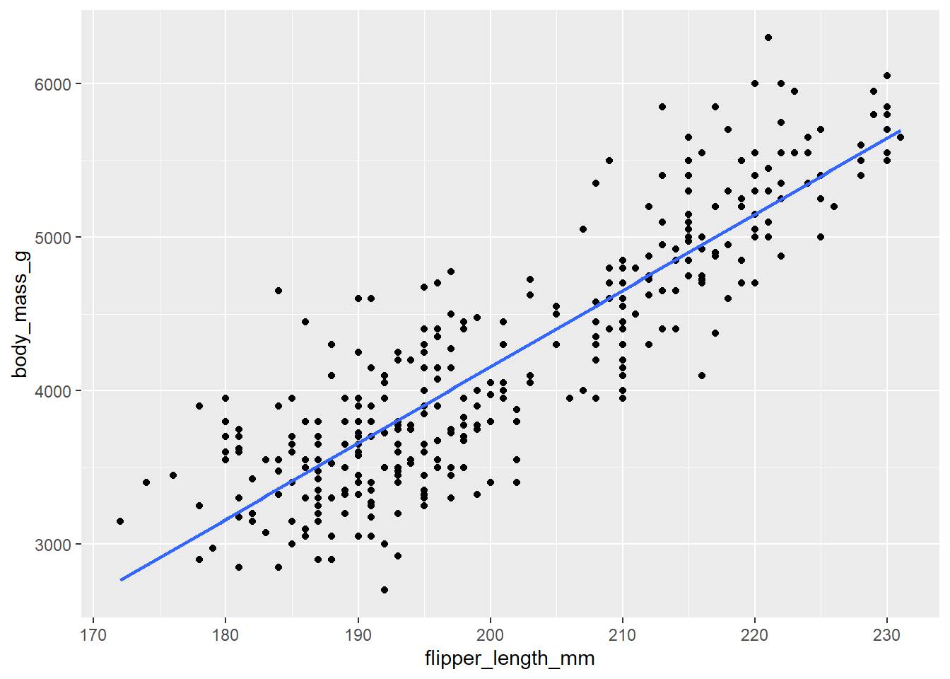
This line estimates the relationship between our two variables. Below, we will practice writing out population and estimated models.
Model these Data
- Write the population model below that explains the relationship between body mass and flipper length.
Hint: You can type equations within dollar signs. LaTeX equations are authored using standard Pandoc markdown syntax (the editor will automatically recognize the syntax and treat the equation as math in the code chunks). It will appear as rendered math in your document.
Useful tips:
“;” is a space in Pandoc markdown
More tips below:
\(x^2 \; superscript\)
\(x_2 \; subscript\)
\(\hat{x}\; adds\; hat\; to\; x\)
\(\beta \; this\; is\; beta\)
\(\epsilon\; this\; is\; epsilon\)
Example:
\(\hat{x^n} + \beta^n = z_n + \epsilon_i\)
\(body_mass = \beta_o + \beta1*flipper_length + \epsilon_i\)
- Now, fit the linear regression model and display the results. Write the estimated model output below.
linear_reg() |>
  set_engine("lm") |>
  fit(body_mass_g ~ flipper_length_mm, data = penguins) |>
  tidy()
# A tibble: 2 × 5
term estimate std.error statistic p.value
<chr> <dbl> <dbl> <dbl> <dbl>
1 (Intercept) -5781. 306. -18.9 5.59e- 55
2 flipper_length_mm 49.7 1.52 32.7 4.37e-107\(\hat{body\_mass} = -5781 + 49.7*flipper_length\)
Interpretation
- Interpret the slope and the intercept in the context of the data.
Hint: Think about what happens to y when we increase x by 1.
Slope: For a 1 mm increase in flipper length, we estimate a mean change of 49.7 grams in body mass.
Intercept: When flipper_length is 0 mm, we estimate a mean body mass of -5791 grams.
Does the intercept make sense? Why or why not? In statistics, what does predicting outside the bounds of our data called?
Extrapolation
Prediction
- What is the estimated mean body mass for a penguin with a flipper length of 210?
-5791 + 49.7*210[1] 4646-5791 + 49.7*100[1] -821