AE 06: Finish AE-05 + AE-06 Suggested Answers

Application exercise

Important

Run the following code until you need to recreate the plot. This is the warm up question for today’s class.

library(tidyverse)

── Attaching packages ─────────────────────────────────────── tidyverse 1.3.2 ──
✔ ggplot2 3.4.0     ✔ purrr   0.3.5
✔ tibble  3.1.8     ✔ dplyr   1.0.9
✔ tidyr   1.2.1     ✔ stringr 1.4.1
✔ readr   2.1.3     ✔ forcats 0.5.2

Warning: package 'ggplot2' was built under R version 4.2.2

Warning: package 'tidyr' was built under R version 4.2.2

Warning: package 'readr' was built under R version 4.2.2

Warning: package 'purrr' was built under R version 4.2.2

── Conflicts ────────────────────────────────────────── tidyverse_conflicts() ──
✖ dplyr::filter() masks stats::filter()
✖ dplyr::lag()    masks stats::lag()

library(scales)


Attaching package: 'scales'

The following object is masked from 'package:purrr':

    discard

The following object is masked from 'package:readr':

    col_factor

fisheries <- read_csv("data/fisheries.csv")

Rows: 82 Columns: 4
── Column specification ────────────────────────────────────────────────────────
Delimiter: ","
chr (1): country
dbl (3): capture, aquaculture, total

ℹ Use `spec()` to retrieve the full column specification for this data.
ℹ Specify the column types or set `show_col_types = FALSE` to quiet this message.

continents <- read_csv("data/continents.csv")

Rows: 245 Columns: 2
── Column specification ────────────────────────────────────────────────────────
Delimiter: ","
chr (2): country, continent

ℹ Use `spec()` to retrieve the full column specification for this data.
ℹ Specify the column types or set `show_col_types = FALSE` to quiet this message.

Global aquaculture production

The Fisheries and Aquaculture Department of the Food and Agriculture Organization of the United Nations collects data on fisheries production of countries.

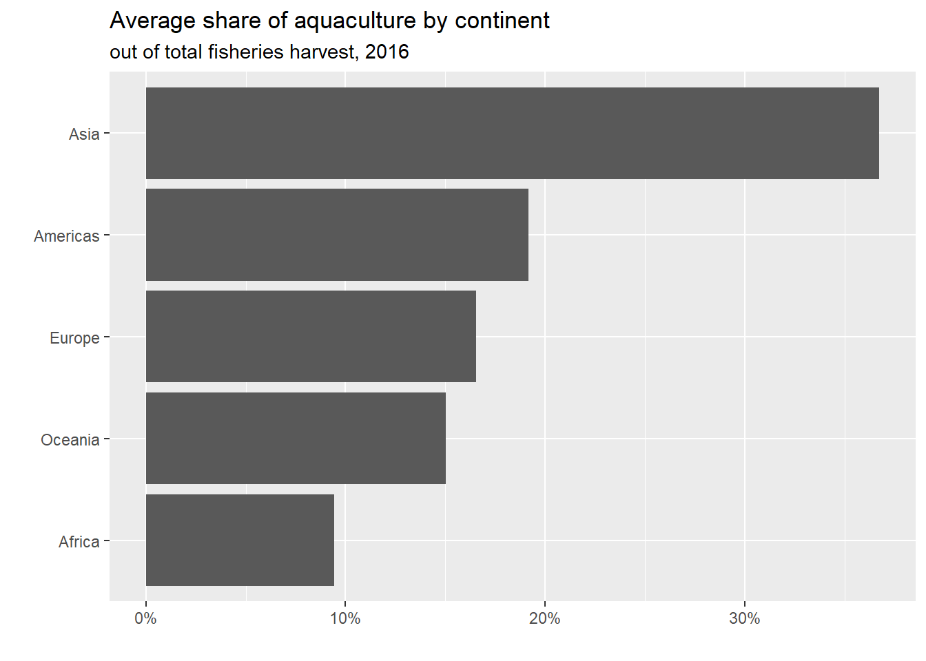
Goal: Our goal is to create a visualization of the mean share of aquaculture by continent.

– Join data sets together

joined_fish <- fisheries |> 
  left_join(continents)

Joining, by = "country"

– Fill in NA values with appropriate continent information

joined_fish <- joined_fish |> 
  mutate(
    continent = case_when(
    country == "Democratic Republic of the Congo" ~ "Africa",
    country == "Hong Kong" ~ "Asia",
    country == "Myanmar" ~ "Asia", 
    TRUE ~ continent
    )
  )

– Add a new column to the joined_fish data frame called aq_prop. We will calculate it as aquaculture / total.

joined_fish <- joined_fish |>
  mutate(aq_prop = aquaculture / total)

Demo: Using your code above, create a new data frame called fisheries_summary that calculates minimum, mean, and maximum aquaculture proportion for each continent in the fisheries data.

fisheries_summary <- joined_fish |>
  group_by(continent) |>
  summarize(
    min_aq_prop = min(aq_prop),
    max_aq_prop = max(aq_prop),
    mean_aq_prop = mean(aq_prop)
  )

Warm up starts here!

Demo: Recreate the following plot using the data frame fisheries_summary you have developed so far.

Hint: We use ftc_relevel to manually specify levels of a factor

We use fct_reorder to reorder a factor based on another variable

We can use functions in R to create more appropriate axis labels (such as adding %s). We can do this through the following: scale_x_continuous(labels = scales::) and scale_y_continuous(labels = scales::). See documentation here and create axis labels that match the picture.

fisheries_summary |>
  ggplot(
    aes(y = fct_reorder(continent, mean_aq_prop),
        x = mean_aq_prop)) + 
  geom_col() + 
  labs(
    title = "Average share of aquaculture by continent",
    subtitle = "out of total fisheries harvest, 2016",
    y =" ",
    x = " "
  ) + 
  scale_x_continuous(labels = scales:: percent)

Pivot Practice

Run the following code below. Are these data in long or wide format? Why?

x <- tibble(
  state = rep(c("MT", "NC" , "SC"),2),
  group = c(rep("C", 3), rep("D", 3)),
  obs = c(1:6)
  )

x

# A tibble: 6 × 3
  state group   obs
  <chr> <chr> <int>
1 MT    C         1
2 NC    C         2
3 SC    C         3
4 MT    D         4
5 NC    D         5
6 SC    D         6

Pivot these data so that the data are wide. i.e. Each state should be it’s own unique observation (row). Save this new data set as y.

y <- x |>
  pivot_wider(names_from = group, values_from = obs)

Now, let’s change it back. Introducing pivot_longer. There are three things we need to consider with pivot_longer:

What the columns will be
names_to
values_to

y |>
  pivot_longer(cols = !state, names_to = "group", values_to = "obs")

# A tibble: 6 × 3
  state group   obs
  <chr> <chr> <int>
1 MT    C         1
2 MT    D         4
3 NC    C         2
4 NC    D         5
5 SC    C         3
6 SC    D         6

Pivot Practice 2

Let’s try this on a real data set.

The Portland Trailblazers are a National Basketball Association (NBA) sports team. These data reflect the points scored by 9 Portland Trailblazers players across the first 10 games of the 2021-2022 NBA season.

trailblazer <- read_csv("data/trailblazer21.csv")

Rows: 9 Columns: 11
── Column specification ────────────────────────────────────────────────────────
Delimiter: ","
chr  (1): Player
dbl (10): Game1_Home, Game2_Home, Game3_Away, Game4_Home, Game5_Home, Game6_...

ℹ Use `spec()` to retrieve the full column specification for this data.
ℹ Specify the column types or set `show_col_types = FALSE` to quiet this message.

– Take a slice at the data. Are these data in wide or long format?

slice(trailblazer)

# A tibble: 9 × 11
  Player Game1…¹ Game2…² Game3…³ Game4…⁴ Game5…⁵ Game6…⁶ Game7…⁷ Game8…⁸ Game9…⁹
  <chr>    <dbl>   <dbl>   <dbl>   <dbl>   <dbl>   <dbl>   <dbl>   <dbl>   <dbl>
1 Damia…      20      19      12      20      25      14      20      26       4
2 CJ Mc…      24      28      20      25      14      25      20      21      27
3 Norma…      14      16      NA      NA      12      14      22      23      25
4 Rober…       8       6       0       3       9       6       0       6      19
5 Jusuf…      20       9       4      17      14      13       7       6      10
6 Cody …       5       5       8      10       9       6       0       7       0
7 Anfer…      11      18      12      17       5      19      17      15      16
8 Larry…       2       8       5       8       3       8       7       0       2
9 Nassi…       7      11       5       9       8       8       4       0       7
# … with 1 more variable: Game10_Home <dbl>, and abbreviated variable names
#   ¹Game1_Home, ²Game2_Home, ³Game3_Away, ⁴Game4_Home, ⁵Game5_Home,
#   ⁶Game6_Away, ⁷Game7_Away, ⁸Game8_Away, ⁹Game9_Home

– Pivot the data so that you have columns for Player, Game, Points. Save this as a new data set called new.blazer.

new.blazer <- trailblazer |>
  pivot_longer(
    cols = !Player,
    names_to = "Game",
    values_to = "Points"
  )

—————————– Answer Below ————————————-

– Suppose now that you are asked to have two separate columns within these data. One column to represent Game, and one to represent Location. Make this happen below. Save your new data set as new.blazer

new.blazer <- trailblazer |>  
  pivot_longer(
    cols = -Player,
    names_to = "Game",
    values_to = "Points",
  ) |> 
  separate(Game, sep = "_", into = c("Game", "Location"))

– Now, use pivot_wider to reshape the new.blazer data frame such that you have a 90 x 4 tibble with columns Player, Game, Home, Away.

new.blazer |>
  pivot_wider(
    names_from = Location,
    values_from = Points
  )

# A tibble: 90 × 4
   Player         Game    Home  Away
   <chr>          <chr>  <dbl> <dbl>
 1 Damian Lillard Game1     20    NA
 2 Damian Lillard Game2     19    NA
 3 Damian Lillard Game3     NA    12
 4 Damian Lillard Game4     20    NA
 5 Damian Lillard Game5     25    NA
 6 Damian Lillard Game6     NA    14
 7 Damian Lillard Game7     NA    20
 8 Damian Lillard Game8     NA    26
 9 Damian Lillard Game9      4    NA
10 Damian Lillard Game10    25    NA
# … with 80 more rows