AE 04: Wrangling flights - Suggest Answers

Application exercise

Important

This AE is due Monday, Jan 30 at 11:59pm.

To demonstrate data wrangling we will use flights, a tibble in the nycflights13 R package. It includes characteristics of all flights departing from New York City (JFK, LGA, EWR) in 2013.

Note: As we go through the AE, practicing thinking in steps, and reading your code as sentences

library(tidyverse)
library(nycflights13) # the data are called flights

finish ae-03 material

`filter()`

Demo: Filter the data frame by selecting the rows where the destination airport is RDU. Save this new data set as RDU_flights. Make sure that this data set only contains the columns dest, year, and carrier.

RDU_flights <- flights |>
  filter(dest == "RDU") |>
  select(dest, year, carrier)

Now, run the following code with one equals sign instead of two. Does it still work?

(=) is a Assignment operator while (==) is a Equal to operator. (=) is used for assigning the values from right to left while (==) is used for showing equality between values.

Demo: We can also filter using more than one condition. Here we select all rows where the destination airport is RDU and the arrival delay is less than 0. As we’ve learned, conditions within functions are separated by a ,.

flights |>
  filter(dest == "RDU", arr_delay < 0)

# A tibble: 4,232 × 19
    year month   day dep_time sched_de…¹ dep_d…² arr_t…³ sched…⁴ arr_d…⁵ carrier
   <int> <int> <int>    <int>      <int>   <dbl>   <int>   <int>   <dbl> <chr>  
 1  2013     1     1      800        810     -10     949     955      -6 MQ     
 2  2013     1     1      832        840      -8    1006    1030     -24 MQ     
 3  2013     1     1      851        851       0    1032    1036      -4 EV     
 4  2013     1     1      917        920      -3    1052    1108     -16 B6     
 5  2013     1     1     1024       1030      -6    1204    1215     -11 MQ     
 6  2013     1     1     1127       1129      -2    1303    1309      -6 EV     
 7  2013     1     1     1157       1205      -8    1342    1345      -3 MQ     
 8  2013     1     1     1317       1325      -8    1454    1505     -11 MQ     
 9  2013     1     1     1505       1510      -5    1654    1655      -1 MQ     
10  2013     1     1     1800       1800       0    1945    1951      -6 B6     
# … with 4,222 more rows, 9 more variables: flight <int>, tailnum <chr>,
#   origin <chr>, dest <chr>, air_time <dbl>, distance <dbl>, hour <dbl>,
#   minute <dbl>, time_hour <dttm>, and abbreviated variable names
#   ¹sched_dep_time, ²dep_delay, ³arr_time, ⁴sched_arr_time, ⁵arr_delay

We can do more complex tasks using logical operators:

operator	definition
`<`	is less than?
`<=`	is less than or equal to?
`>`	is greater than?
`>=`	is greater than or equal to?
`==`	is exactly equal to?
`!=`	is not equal to?
`x & y`	is x AND y?
`x \\| y`	is x OR y?
`is.na(x)`	is x NA?
`!is.na(x)`	is x not NA?
`x %in% y`	is x in y?
`!(x %in% y)`	is x not in y?
`!x`	is not x?

The final operator only makes sense if x is logical (TRUE / FALSE).

Your turn (4 minutes): Describe what the code is doing in words.

flights |> # Data set 
  filter(dest %in% "RDU", # Is RDU in dest?
         arr_delay < 0 | dep_delay < 0
         ) |>
  glimpse()

What if we want to like at destinations of RDU and GSO? How does the below code change?

  flights |>
  filter(dest %in% c("RDU", "GSO"),
         arr_delay < 0 | dep_delay < 0
         )

# A tibble: 6,203 × 19
    year month   day dep_time sched_de…¹ dep_d…² arr_t…³ sched…⁴ arr_d…⁵ carrier
   <int> <int> <int>    <int>      <int>   <dbl>   <int>   <int>   <dbl> <chr>  
 1  2013     1     1      800        810     -10     949     955      -6 MQ     
 2  2013     1     1      832        840      -8    1006    1030     -24 MQ     
 3  2013     1     1      851        851       0    1032    1036      -4 EV     
 4  2013     1     1      917        920      -3    1052    1108     -16 B6     
 5  2013     1     1     1024       1030      -6    1204    1215     -11 MQ     
 6  2013     1     1     1127       1129      -2    1303    1309      -6 EV     
 7  2013     1     1     1157       1205      -8    1342    1345      -3 MQ     
 8  2013     1     1     1317       1325      -8    1454    1505     -11 MQ     
 9  2013     1     1     1449       1450      -1    1651    1640      11 MQ     
10  2013     1     1     1505       1510      -5    1654    1655      -1 MQ     
# … with 6,193 more rows, 9 more variables: flight <int>, tailnum <chr>,
#   origin <chr>, dest <chr>, air_time <dbl>, distance <dbl>, hour <dbl>,
#   minute <dbl>, time_hour <dttm>, and abbreviated variable names
#   ¹sched_dep_time, ²dep_delay, ³arr_time, ⁴sched_arr_time, ⁵arr_delay

Why c?

combine: Use when we create a list

Your turn (2 minutes): Subset the data to only include planes that traveled more than 500 in distance and had a negative departure delay.

flights |>
  filter(distance > 500 & dep_delay < 0)

# A tibble: 137,888 × 19
    year month   day dep_time sched_de…¹ dep_d…² arr_t…³ sched…⁴ arr_d…⁵ carrier
   <int> <int> <int>    <int>      <int>   <dbl>   <int>   <int>   <dbl> <chr>  
 1  2013     1     1      544        545      -1    1004    1022     -18 B6     
 2  2013     1     1      554        600      -6     812     837     -25 DL     
 3  2013     1     1      554        558      -4     740     728      12 UA     
 4  2013     1     1      555        600      -5     913     854      19 B6     
 5  2013     1     1      557        600      -3     838     846      -8 B6     
 6  2013     1     1      558        600      -2     753     745       8 AA     
 7  2013     1     1      558        600      -2     849     851      -2 B6     
 8  2013     1     1      558        600      -2     853     856      -3 B6     
 9  2013     1     1      558        600      -2     924     917       7 UA     
10  2013     1     1      558        600      -2     923     937     -14 UA     
# … with 137,878 more rows, 9 more variables: flight <int>, tailnum <chr>,
#   origin <chr>, dest <chr>, air_time <dbl>, distance <dbl>, hour <dbl>,
#   minute <dbl>, time_hour <dttm>, and abbreviated variable names
#   ¹sched_dep_time, ²dep_delay, ³arr_time, ⁴sched_arr_time, ⁵arr_delay

`count()`

Demo: Create a frequency table of the destination locations for flights from New York.

flights |> 
  count(dest)

# A tibble: 105 × 2
   dest      n
   <chr> <int>
 1 ABQ     254
 2 ACK     265
 3 ALB     439
 4 ANC       8
 5 ATL   17215
 6 AUS    2439
 7 AVL     275
 8 BDL     443
 9 BGR     375
10 BHM     297
# … with 95 more rows

Demo: In which month was there the fewest number of flights? How many flights were there in that month? Hint: Type ?min into the console.

flights |>
  count(month) |>
  filter(n == min(n))

# A tibble: 1 × 2
  month     n
  <int> <int>
1     2 24951

On which date (month + day) was there the largest number of flights? How many flights were there on that day?

flights |> 
  count(month,day) |>
  filter(n == max(n))

# A tibble: 1 × 3
  month   day     n
  <int> <int> <int>
1    11    27  1014

`mutate()`

Use mutate() to create a new variable.

Demo: In the code chunk below, air_time (minutes in the air) is converted to hours, and then new variable mph is created, corresponding to the miles per hour of the flight. Run the code. Next, comment each line of code below.

flights |> 
  mutate(hours = air_time / 60, 
         mph = distance / hours) |>
  select(air_time, distance, hours, mph)

# A tibble: 336,776 × 4
   air_time distance hours   mph
      <dbl>    <dbl> <dbl> <dbl>
 1      227     1400 3.78   370.
 2      227     1416 3.78   374.
 3      160     1089 2.67   408.
 4      183     1576 3.05   517.
 5      116      762 1.93   394.
 6      150      719 2.5    288.
 7      158     1065 2.63   404.
 8       53      229 0.883  259.
 9      140      944 2.33   405.
10      138      733 2.3    319.
# … with 336,766 more rows

Your turn (4 minutes): Create a new variable to calculate the percentage of flights in each month. What percentage of flights take place in July?

flights |>
  count(month) |>
  mutate(perc = n / sum(n) * 100)

# A tibble: 12 × 3
   month     n  perc
   <int> <int> <dbl>
 1     1 27004  8.02
 2     2 24951  7.41
 3     3 28834  8.56
 4     4 28330  8.41
 5     5 28796  8.55
 6     6 28243  8.39
 7     7 29425  8.74
 8     8 29327  8.71
 9     9 27574  8.19
10    10 28889  8.58
11    11 27268  8.10
12    12 28135  8.35

changing variable type

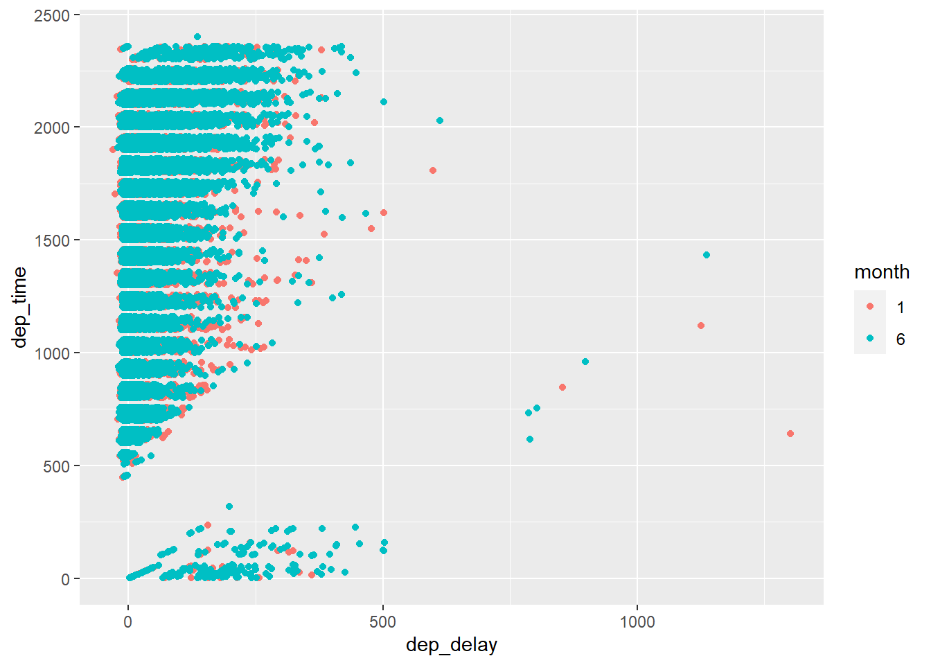
Your turn (5 minutes): We want to create a visualization to assess the relationship between dep_delay and dep_time conditioned on the months January and June. Using the code chunk below, check to see which types of variables each of the three listed above are. Next, create an appropriate visualization to answer the question above. Hint: You may have to change the type of one variable using factor. Comment each line of code below.

flights |>
  filter(month %in% c(1 , 6)) |>
  mutate(month = factor(month)) |>
  #droplevels() |>
  ggplot(
    aes(x = dep_delay, y = dep_time, color = month)
  ) + 
  geom_point()

Warning: Removed 1530 rows containing missing values (`geom_point()`).

`summarize()`

summarize() collapses the rows into summary statistics and removes columns irrelevant to the calculation.

Be sure to name your columns!

Calculate the mean departure delay below.

flights |> 
  summarize(mean_dep_delay = mean(dep_delay))

# A tibble: 1 × 1
  mean_dep_delay
           <dbl>
1             NA

Question: Why did this code return NA?

Let’s fix it! We can use na.rm to remove NAs.

flights |> 
  summarize(mean_dep_delay = mean(dep_delay, na.rm = F))

`group_by()`

group_by() is used for grouped operations. It’s very powerful when paired with summarise() to calculate summary statistics by group.

Here we find the mean and standard deviation of departure delay for each month. Comment each line of code below.

flights |> 
  group_by(month) |> # groups together all observations that have the same month
  summarize(mean_dep_delay = mean(dep_delay, na.rm=T), #calculate mean
            sd_dep_delay = sd(dep_delay, na.rm=T) #calculate sd
            )

# A tibble: 12 × 3
   month mean_dep_delay sd_dep_delay
   <int>          <dbl>        <dbl>
 1     1          10.0          36.4
 2     2          10.8          36.3
 3     3          13.2          40.1
 4     4          13.9          43.0
 5     5          13.0          39.4
 6     6          20.8          51.5
 7     7          21.7          51.6
 8     8          12.6          37.7
 9     9           6.72         35.6
10    10           6.24         29.7
11    11           5.44         27.6
12    12          16.6          41.9

Your turn (4 minutes): What is the median departure delay for each airports around NYC (origin)? Which airport has the shortest median departure delay?

flights |>
  group_by(origin) |>
  summarize(med_dep_delay = median(dep_delay, na.rm = T))

Optional

Create a new data set that only contains flights that do not have a missing departure time. Include the columns year, month, day, dep_time, dep_delay, and dep_delay_hours (the departure delay in hours). Hint: Note you may need to use mutate() to make one or more of these variables.

new.data <- flights |>
  filter(!is.na(dep_time)) |>
  select(dep_time, dep_delay) |>
  mutate(dep_delay_hours = dep_delay / 60)

For each airplane (uniquely identified by tailnum), use a group_by() paired with summarize() to find the sample size, mean, and standard deviation of flight distances. Then include only the top 5 and bottom 5 airplanes in terms of mean distance traveled per flight in the final data frame.

flights |>
  group_by(tailnum) |>
  summarize(n = n(),
            mean = mean(distance),
            sd = sd(distance)) |>
  arrange(desc(mean)) |>
  slice(c(1:5, (n()-4):n()))

# A tibble: 10 × 4
   tailnum     n  mean    sd
   <chr>   <int> <dbl> <dbl>
 1 N380HA     40 4983    0  
 2 N381HA     25 4983    0  
 3 N382HA     26 4983    0  
 4 N383HA     26 4983    0  
 5 N384HA     33 4983    0  
 6 N945UW    285  176.  31.2
 7 N956UW    222  174.  31.4
 8 N959UW    213  174.  34.3
 9 N948UW    232  174.  32.7
10 N955UW    225  173.  32.9